Identification of Incorrect Data Labels Using Conditional Outlier Detection

1. INTRODUCTION

With the spread of social network services and online media platforms, the availability of user- created data content increases drastically. These data are often accompanied by human-annotated labels, such as tags associated with images or vid- eos, topic words assigned to Web articles, and ti- tles given to sound clips, etc. In terms of data ac- cessibility, such annotations are generally found to be useful in that they provide a brief idea of data content and can be utilized to design another in- formation retrieval service.

As for the data labels annotated by human, how- ever, those tags or keywords sometimes contain errors in that they are mistakenly selected by the user and irrelevantly matched with the data.

Apparently, identifying and removing those erratic

labels in user-annotated data are one of the im- portant steps in data preprocessing, when one con- siders utilizing the data for any purpose. One way to analyze and discover such mistakes in data is outlier (or anomaly) detection. Outlier detection is a data analytic task that pursues to find unusual instances in a dataset [1-4]. It has been an active research topic in data science and artificial in- telligence communities and frequently used in var- ious applications to identify rare and interesting data patterns that may be associated with either beneficial or malicious events such as fraud identi- fication [5, 6], network intrusion surveillance [7, 8], disease outbreak detection [9], patient monitoring for preventable adverse events (PAE) [10, 11], etc.

It is also utilized as a primary data preprocessing step that helps to remove noisy or irrelevant sig- nals in data [12, 13].

Identification of Incorrect Data Labels Using Conditional Outlier Detection

Charmgil Hong

^†

ABSTRACT

Outlier detection methods help one to identify unusual instances in data that may correspond to erroneous, exceptional, or surprising events or behaviors. This work studies conditional outlier detection, a special instance of the outlier detection problem, in the context of incorrect data label identification.

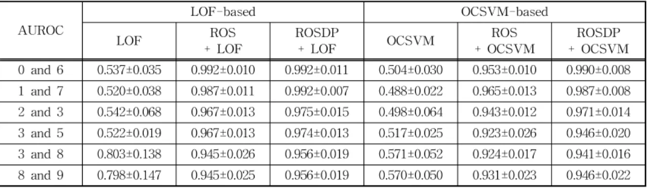
Unlike conventional (unconditional) outlier detection methods that seek abnormalities across all data attributes, conditional outlier detection assumes data are given in pairs of input (condition) and output (response or label). Accordingly, the goal of conditional outlier detection is to identify incorrect or unusual output assignments considering their input as condition. As a solution to conditional outlier detection, this paper proposes the ratio-based outlier scoring (ROS) approach and its variant. The propose solutions work by adopting conventional outlier scores and are able to apply them to identify conditional outliers in data. Experiments on synthetic and real-world image datasets are conducted to demonstrate the benefits and advantages of the proposed approaches.

Key words: Conditional Outlier Detection, Outlier Analysis, Anomaly Detection

※ Corresponding Author : Charmgil Hong, Address:

(37554) Handong-ro 558, Buk-gu, Pohang, Gyeongbuk, Korea, TEL : +82-10-2663-9088, FAX : +82-54-260- 1309, E-mail : [email protected]

Receipt date : Jul. 10, 2020, Approval date : Jul. 20, 2020

†School of Computer Science and Electrical Engineering, Handong Global University

This work considers conditional outlier de- tection (COD) [10, 14] and proposes a novel ap- proach to identify errors or mistakes in the annota- tion space. COD is a special case of the outlier de- tection problem that aims to find data objects with unusual values for a subset of variables given the values of the remaining variables. COD is partic- ularly useful when data is considered to manifest conditional dependences among its variables; i.e., a set of variables defines context (input), while the rest are treated as response given the context.

Unlike conventional (unconditional) outlier detec- tion methods that seek abnormalities across all da- ta attributes, COD examines and looks for data in- stances with unusual pairing of input and output values. Accordingly, in the problem of unusual im- age tags (labels) identification, the COD approach could be especially useful as the approach directly considers the annotation (output) space given as- sociated data instance (input).

Despite its importance and usefulness, COD has received relatively less attention, while the ma- jority of existing research have focused on uncon- ditional outliers [2, 15]. However, as conditional outliers are fundamentally different from uncondi- tional outliers in that conditional outliers reflect unusual responses for a given set of contextual at- tributes, applications of unconditional outlier de- tection methods to a COD problem may lead to in- correct results. For instance, consider where one wants to find mistaken image tags in a collection

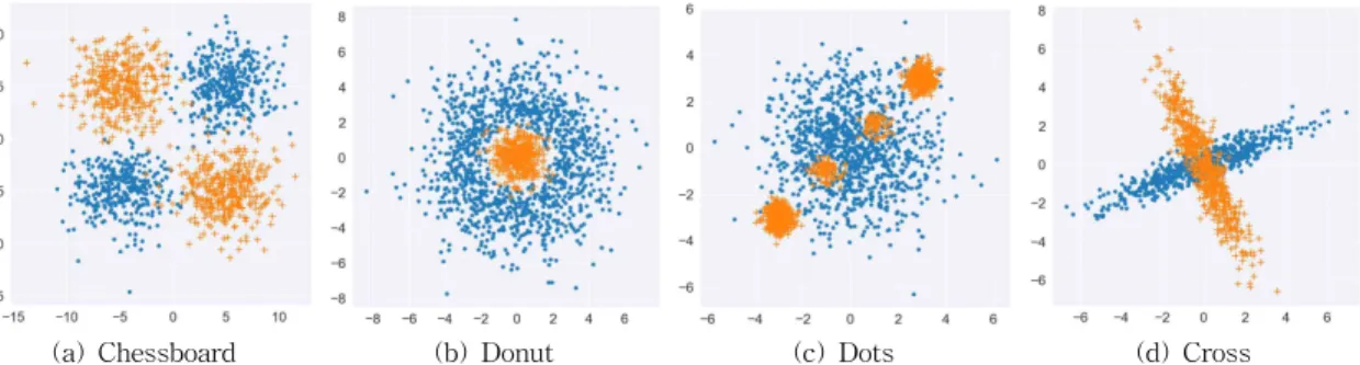
of annotated images. If an unconditional outlier de- tection method is applied jointly to both images and tags, images with rare themes may get flagged in- stead of images with mistaken tags (false pos- itives) due to the scarcity of the themes in the dataset. Similarly, images with frequent themes but with unusual annotations may not be detected as outliers due to the abundance of similar themes in the dataset (false negative). Fig. 1 illustrates a COD problem with image-annotation pairs.

This paper proposes a new COD solution that works by comparing (via ratio) two unconditional outlier scores: one score calculated against data with the same observed output value; and another calculated against data with the opposite output value. This new approach offers a couple of merits in addressing the COD problem. First, it allows the user to utilize a wide variety of unconditional out- lier scores. Second, it lets one effectively avoid the cases where instances with rare observation but properly associated with the output undesirably re- ceive a high conditional outlier score. Through the paper, the derivation and development of the meth- od is explained. With experiments, the performance and usefulness of the proposed method is demon- strated.

The rest of the paper is organized as follows.

Section 2 revisits the background of conditional outlier detection and relevant research work.

Section 3 presents the new COD framework and discuss its properties. Section 4 compares and

Fig. 1. Examples of conditional outliers. In this example, each data instance contains an image of handwritten digit

[16] and a user-annotated label. Data instances marked with dotted (red) rectangles represent conditional

outliers that are annotated with unusual or incorrect labels compared to the rest.

demonstrates the performance of the proposed solution. Section 5 concludes the paper.

2. BACKGROUND

2.1 Problem Definition: Conditional Outlier Detection (COD)

Given dataset ^{  x}

^{ }

^

^{ }

^

n  

N

, where x∈ℝ

^m

and ^{∈} , conditional outliers are the outliers that occur in the output space ( ^ ) conditioned on the input ( ^X ). That is, the goal in conditional out- lier detection (COD) is to identify data instances that have unusual output value given their input.

This special type of outlier detection problem is challenging because the dependence relations be- tween input and output should be taken into ac- count when identifying outliers. The following subsections review the relevant research and pin- point the main differences that the proposed ap- proach has.

2.2 Conditional Outlier Detection

Conventionally COD for discrete output space is addressed by modeling the posterior distribution and by identifying data objects that do not fit well the model. In other words, data objects that are as- signed a very low posterior probability are consid- ered conditional outliers. Accordingly, depending on how to represent the posterior, a number of methods have been proposed. Hauskrecht et al. [10]

is one of the earliest work that introduced the con- cept and importance of the conditional approach to the outlier problem. The authors used a localized Bayesian networks to represent data with discrete input and output variables. The same group [11, 17] further developed the framework to address COD with mixture of continuous and discrete inputs. Valko and Hauskrecht [18] investigated the instance-specific methods to acquire more accu- rate predictive models for COD. To select instances that are similar to the target instance, the authors presented a new metric learning algorithm.

Although the abovementioned methods directly tackled the COD problem, they are different from the approach proposed in this paper, in that the ex- isting methods are based on specially designed da- ta models or algorithms for conditional outlier de- tection. This work proposes a solution that works by adopting existing unconditional outlier detection methods.

2.3 Unconditional Outlier Detection

While the COD problem has been the focus of some recent research efforts, its unconditional counterpart has long been investigated as the main area of the outlier detection research. One way to summarize existing unconditional methods is to organize them according to the assumptions that each method builds upon. Out of many, the dis- cussion conducted in this paper is directly relevant to the following categories of methods.

∙ Density-based approaches: Density-based approaches assume that the density around a nor- mal data instance is similar to the density around its neighbors, while that of an outlier is relatively lower than its neighbors. Local Outlier Factor (LOF) [19] is one of the most popular methods in this category. LOF has shown a good performance in many applications and is considered as an off-the-shelf outlier detection method. Section 3.1.1 reviews this method more in detail and dis- cusses how to combine LOF with the proposed approach.

∙ Classification-based approaches: Classifica-

tion-based approaches are based on a parametric

assumption that a function of feature classifying

normal and outlier instances can be learned from

data. One-class classification strategy is a popular

technique falls in this category. It assumes that all

training instances are normal, and attempts to

learn a discriminative boundary around the training

(normal) instances. For testing, instances that fall

out of the obtained decision boundary are consid-

ered to be outliers. Support vector machines (SVMs) have been applied to outlier detection us- ing this strategy [20]. Section 3.1.2 reviews this approach and discusses how it is combined in the proposed solution.

2.4 Ensemble Approach to Outlier Detection The approach proposed in this work can be seen as an ensemble approach in that it combines un- conditional outlier scores and weaves them into a conditional outlier score. There have been several work in this direction in the purpose of improving the overall (unconditional) outlier detection per- formance [21, 22]. However, to the best of knowl- edge, there has been no conditional outlier detection method that can is based on an ensemble approach.

3. PROPOSED METHOD

3.1 Ratio of Outlier Scores (ROS)

This paper proposes a new conditional outlier detection approach that works by comparing two unconditional outlier scores and forming a ra- tio-like score: One score is calculated against data with the same observed output value; Another cal- culated against data with the opposite output value.

This new score is referred to as Ratio of Outlier Scores (or Ratio-based Outlier Scoring; ROS). It offers a couple of important advantages. First, it allows to utilize a wide variety of unconditional outlier scores. Also, it lets one effectively avoid the cases where instances with rare observation but properly associated with the output undesirably re- ceive a high conditional outlier score.

More formally, consider a binary-labeled dataset

  x

^{ }



^{ }



_{  }^

where each instance in ^ con- sists of a continuous input vector ^x

^{ }

^∈ℝ

^

, and an associated output value ^

^{ }

^{ } . For notational convenience, ^

  

and ^

  

are defined to denote subsets of  based on the value of ^

^{ }

:



_{  }

 x

^

 

^{ }



A subset of ^ whose output value is equal to



^{ }

( ^

  

does not include the n-th instance)



  

 x

^

≠ 

^{ }



A subset of ^ whose output value is not equal to ^

^{ }

Then, for the n-th data instance ^x

^{ }

^

^{ }

^ ,



_{R O S}



^{ }

x

^{ }

 is defined as the ratio between two unconditional outlier scores evaluated on



_{  }

and ^

  

, respectively:



_{R O S}



^{ }

x

^{ }

　   

_

x

^{ }



  





_

x

^{ }



_{  }



(1)

where ^





^{ }

 denotes an unconditional outlier score computed for ^x

^{ }

on dataset ^ .

ROS measures the unusualness of the input ^x

^{ }

being associated with its output ^

^{ }

. For normal data instances ^{}

R O S



^{ }

x

^{ }

 would be low, which in turn indicates the outlier score based on



_{  }

is low and/or ^

  

is high. On the other hand, instances with a high ROS score are deemed as outliers, because ^{}

R O S



^{ }

x

^{ }

 is high when the outlier score based on ^

  

is high and/or ^

  

is low.

Note that Equation (1) easily turns many exist-

ing unconditional outlier scores to conditional out-

lier scores. That is, it can compute and compare

the conditional outlier score of data instances by

simply applying any unconditional outlier score -

such as density-based outlier scores [19, 23], clas-

sification-based outlier scores [20, 24], etc. - to the

subsets of  and computing their ratio. Another

advantage of this approach is that it can properly

handle instances that fall in regions of the input

space with low support. For a data instance that

does not have enough support (i.e., an instance falls

in a sparse neighborhood of ^X ), it is not straight-

forward to come up with an outlier score that is

confident. However, the proposed score suffers less

from the issue, because both ^

  

and ^

  

will be high in such a sparse region and, as a result, by cancelling each other out in Equation (1), the resulting conditional outlier score will not be high.

In summary, the new conditional outlier de- tection approach based on the ratio-score defines a general and flexible framework that allows one to plug in an unconditional outlier score and use it to perform conditional outlier detection. The next subsections (Sections 3.1.1 and 3.1.2) introduce how to use ROS in combination with the Local Outlier Factor (LOF) and One-Class Support Vec- tor Machine (OCSVM) methods and their defi- nitions [19, 20].

3.1.1 ROS with Local Outlier Factor (LOF) Recall that LOF [19] is a non-parametric ap- proach used to detect unconditional outliers based on the density of the local neighborhood of the tar- get data instance. More specifically, it computes the outlier score of an instance by comparing the local density of the instance to the average local density of its ^ nearest neighbors:



_

x

^{ }

  x

^{ }

     

_

x

^{ }

 

x^∈ 



x^ 

 

_

x

^{ }





_

x

^



(2) where ^

_

^x

^{ }

 denotes the unconditional outlier score for instance ^x

^{ }

and dataset ^ ,  

_

x

^{ }

 

denotes the ^ -nearest neighbors of instance ^x

^{ }

in dataset ^ , and



_

ξ  

∈



_ξ 

max

_

ξ

 ^



ξ 

(3)

is the local reachability density, which measures the geometric dispersion of the ^ -nearest neigh- borhood, where ^{ξ} denotes the distance be- tween two instances ^ and ^ ; and ^



 denotes the distance to the ^ -th nearest neighbor of  . In this work the Mahalanobis distance is used to compute the pairwise distances.

To come up with the ROS score, Equation (2)

is estimated against 

_{  }

and 

  

, re- spectively, and the ratio of the two scores is com- puted (Equation (1)).

3.1.2 ROS with One-Class Support Vector Machine (OCSVM)

OCSVM is a classification-based method origi- nally designed to detect unconditional outliers [20].

It trains an SVM classifier by learning a decision boundary between training data and the origin (zero). Any instances that lie across the boundary are classified as outliers. To compute the ROS score using OCSVM, two SVM models are trained separately on 

_{  }

and 

  

, and define decision boundaries for unconditional outliers.

Then the ratio between the raw scores estimated both models are used for conditional outlier detec- tion.

3.2 ROS on Discriminative Projections

The above newly designed conditional outlier score leverages the ratio of two unconditional out- lier scores that are computed in the input space.

Hence, any issues affecting the quality of the un- conditional scores are likely to be inherited to the new ratio score.

One of the recurring challenges of many uncon- ditional outlier detection approaches is that they tend to exhibit poor performance when the data di- mensionality is high. This is because in high-di- mensional data spaces, with many (random) di- mensions, all data objects appear to be sparse, and many of the distance metrics and density estima- tors become analytically ineffective and computa- tionally intractable [25-27]. As a result, outliers become hard to define and detect. It is reasonable to assume that these limitations also translate to the conditional score when it comes to the proposed ratio outlier score, and devising a solution to im- prove the robustness of the method is appropriate.

One common way to resolve the problem of a

high-dimensional space (in unconditional settings)

is to reduce the dimensionality of the space via various dimensionality reduction methods, such as principal component or independent component analysis [28, 29], before the detection. However, the conditional outlier detection is different, as the im- portance of the input space and its individual di- mensions depends on how important the dimen- sions are in defining (or predicting) the output. In such a case, various supervised space trans- formations or supervised metric learning appro- aches can be applied.

To cope with the dimensionality problem, this work adopts a relatively simple supervised di- mensionality reduction approach that relies on a discriminative model and its output to define a lower-dimensional projection of the original (high- dimensional) input data. In principle, one can use one or more such discriminative projections. This work focuses on and experiments with one-dimen- sional projections, in which a high-dimensional in- put space is reduced to a one-dimensional discrim- inative space. Such projections can be built with the help of various classification learning methods.

For example, by applying the logistic regression model to the dataset ^ , a probabilistic projection of ^x

^{n }

^y

^{n }

^ representing ^{  }

^{ }

^{X  x}

^{n }

^ is obtained. Similarly, by taking a raw output of a support vector machines model, non-probabilistic discriminative projections are obtained. Below de- notes such a discriminative projection function as

 and the projection of the function as φ.

  x

^{ }

→ 

^{ }

(4)

Obtaining a discriminative projection function ^ and its projections φ is equivalent to training (learning) of a model on the input-output instances in  . Assuming the logistic regression model, the parameters of the projection function are optimized as:



_

 argmax

_{n  }



^N

^log

^{ }

^x

^{n }

^{ (5)}

After ^



is obtained from data, the projection

function ^ on an observed input ^x

^{ }

as follows:



^{ }

 x

^{n }

     exp x

^{n }



_f



 (6)

To combine the discriminative projections with the ROS approach, firstly the original data is map- ped to the projected discriminative space. After that, the ROS scores are computed on the newly projected space. This extension of ROS is referred to as Ratio of Outlier Scores on Discriminative Projections (ROSDP) approach. To formalize, giv- en the parameters of the discriminative projection

 , the ROSDP score is defined as:



_{R O SD P}



^{ }

x

^{ }

　  (7)

 

_

x

^{ }



  





_

x

^{ }



_{  }



  

_



^{ }



  





_



^{ }



_{  }



where



_{   }

 

^



^

 

^{ }

A subset of the projections of ^ on ^ whose output value is equal to ^

^{ }

( ^

  

does not include ^

^{ }

)



_{ }  

 

^



^

≠

^{ }

A subset of the projections of ^ on ^ whose output value is not equal to ^

^{ }

In the following section, the advantages of the proposed conditional outlier approach based on the ROS score and its combination with discriminative projections (ROSDP) approach are demonstrated through experiments.

4. EXPERIMENTAL STUDY

To validate the correctness and effectiveness of

the proposed methods, this section performs an ex-

perimental study with synthetic and real world

datasets. Recall that both ROS and ROSDP are

meta-methods in that they are designed to adopt

and interplay with unconditional outlier detection

methods. As reviewed and discussed in Sections

3.1.1 and 3.1.2, this work utilizes the local outlier factor (LOF) and one-class support vector ma- chine (OCSVM) methods for experiments. In par- ticular, the experiments conducted in this section compare the following methods:

∙ Local Outlier Factor on the Joint Space (LOF) [19] - This applies LOF (Equation (2)) to the joint space of all data attributes (both input and output)

∙ Ratio of Outlier Scores with LOF (ROS+LOF) – This evaluates the ratio-based outlier score (Equation (1)) with LOF calculated on the original input space

∙ Ratio of Outlier Scores on Discriminative Projection with LOF (ROSDP+LOF) - This eval- uates the ratio-based outlier score with LOF on a discriminative projection space (Equation (7))

∙ One-Class Support Vector Machine on the Joint Space (OCSVM) [20] - This applies OCSVM (Section 3.1.2) to the joint space of all data attrib- utes (both input and output)

∙ Ratio of Outlier Scores with OCSVM (ROS+

OCSVM) – This evaluates the ratio-based outlier score (Equation (1)) with OCSVM applied to the original input space

∙ Ratio of Outlier Scores on Discriminative Projection with LOF (ROSDP+LOF) - This eval- uates the ratio-based outlier score with OCSVM applied to a discriminative projection space (Equa- tion (7))

For every instance of LOF (LOF, ROS+LOF, and ROSDP+LOF), we set the number of neighbors to k = 50; and use Mahalanobis distance to measure the distance between pairs of instances. To obtain data models/discriminative projection functions in ROSDP, we use L

2

-regularized logistic regression and choose the regularization coefficient using the internal cross validation.

4.1 Experiment Setup

The evaluation and comparisons of COD meth- ods could be very challenging because outlier vali- dation may be ambiguous and may require addi-

tional human feedback. For the purpose of the comparative evaluation, this work conducts ex- periments on simulated outliers as follows:

1. In each experiment, select 1.0% of instances uniformly at random (outlier ratio = 1.0%)

2. For each selected instance, invert the output value ( ^

 

 

_{ }

  )

The resulting outliers can be interpreted as con- textually abnormal output signals, that could be considered as errors or mistakes. For example, in an annotated image dataset, the outliers would be perceived as images with incorrect labels.

It should be stressed out that all methods in be- low experiments (including their model building and outlier scoring stages) are run on data with simulated outliers. In other words, the models are not trained on the clean (i.e., outlier-free) data be- fore they perform outlier detection on the data with simulated outliers. Such a setup is indeed im- practical since in real world applications outliers in data are not a priori known nor cannot be excluded.

4.2 Evaluation Metrics

This work uses the Area Under the Precision- Recall Curve (AUPRC) as the primary performance measure. AUPRC summarizes the precision-recall tradeoff in all range of outlier scores. In the context of outlier detection, precision measures how much outlier calls are correct out of all outlier calls made;

Recall measures how much outliers are correctly detected out of all outliers in data.

This work also evaluates the Area Under the Receiver Operating Characteristic Curve (AUROC).

AUROC summarizes the specificity-recall tradeoff

over all possible outlier detection thresholds. Al-

though AUROC has been a widely used metric for

outlier detection performance, it is worthwhile to

note that the metric is not precisely reflecting the

outlier detection performance as AUROC puts true

negatives (normal instances that are identified to

be normal) in evaluation. As normal (non-outlying)

data instances are usually dominant in a dataset, AUROC tends to overestimate the outlier detection performance.

For both AUPRC and AUROC, higher means better performance.

4.3 Experiments

4.3.1 Synthetic Data (Identification of Unusual Data Labels)

Data Four synthetic datasets are used for the evaluation of outlier detection performance. Each artificial dataset contains 2,000 instances of 2-di- mensional continuous input ( ^{X ∈ℝ}

^

) and binary ( ^{  } ) output pair that form a unique shape as displayed in Fig. 2. In Fig. 2, the inputs (context) are the coordinates, while the binary outputs (responses) are denoted in shapes (0=blue circle, 1=orange cross). For convenience, the datasets are referred to as Chessboard (Fig. 2(a)), Donut (Fig.

2(b)), Dots (Fig. 2(c)), and Cross (Fig. 2(d)).

Simulating Outliers Conditional outliers are simulated by selecting 1.0% of the dataset in- stances and by inverting their output labels (recall Section 4.1). Given that each dataset contains two classes representing the membership, the simu- lated outliers can be interpreted as incorrect re- sponse in the output space (wrongful class assign- ments).

Results Tables 1 and 2 summarize the results on the four synthetic datasets. All the results are averaged over five simulation runs. The numbers shown in boldface in the tables indicate the best results (by paired t-test at α = 0.05) on each ex- periment set.

In terms of AUPRC (Table 1), ROS+LOF and ROSDP+LOF are the clear winners. Across all ex- periments, ROS+LOF and ROSDP+LOF detect conditional outliers with statistically superior per- formances. Compared to LOF, the base outlier

(a) Chessboard (b) Donut (c) Dots (d) Cross

Fig. 2. Synthetic datasets for experiments. The inputs (context) are the coordinates, while the binary outputs (responses) are denoted in shapes (0=blue circle, 1=orange cross). According to the shape, the datasets are referred to as: (a) Chessboard, (b) Donut, (c) Dots, and (d) Cross.

Table 1. Area Under the Precision-Recall Curve (AUPRC)

AUPRC

LOF-based OCSVM-based

LOF ROS

+ LOF ROSDP

+ LOF OCSVM ROS

+ OCSVM ROSDP

+ OCSVM

Chessboard 0.429±0.016 0.945±0.018 0.938±0.020 0.052±0.008 0.881±0.024 0.932±0.018

Donut 0.131±0.022 0.464±0.060 0.463±0.059 0.034±0.007 0.098±0.016 0.085±0.010

Dots 0.098±0.016 0.376±0.051 0.395±0.051 0.030±0.004 0.032±0.003 0.028±0.002

Cross 0.145±0.021 0.575±0.067 0.559±0.068 0.039±0.008 0.471±0.055 0.407±0.044

Numbers shown in bold indicate the best results on each experiment set (by paired t-test at α=0.05).

score estimator of the former, there is a huge im- provement that highlights the usefulness of the proposed ratio-based approach. Although not as good as ROS+LOF and ROSDP+LOF, the ROS methods combined with OCSVM also produce strong results. On two of the synthetic datasets, ROS+OCSVM and ROSDP+OCSVM show superi- or performances. On the Donut and Dots datasets, however, the improvement is not as evident. This is because the input regions of each output value are not as separate as in the other dataset and. in turn, OCSVM applied to each class does not yield distinctive scores for the ratio-based estimation.

A similar performance pattern is observed in terms of AUROC (Table 2), while the performance difference between methods are not as apparent as with AUPRC. Across all four datasets, ROS+LOF and ROSDP+LOF always outperform the other methods, and ROS+OCSVM and ROSDP+OCSVM follow. On the other hand, the base estimators, LOF and OCSVM, applied to the joint space of in- put and output, do not produce meaningful results in terms of conditional outlier detection. Overall, the experimental results support the proposed framework for conditional outlier detection.

4.3.2 Real World Image Data (Identification of Incorrect Image Annotations)

Data The data used in this section is the MNIST dataset [16]. This dataset contains images of hand-written digits (as in Fig. 3), along with the ground truth labels telling what digits are

scanned. In particular, six subsets of MNIST are used for the experiments; each subset includes 2,000 randomly sampled images of two pre-se- lected digits (1,000 images per digit). The pre-se- lected pairs of digits are:

∙ 0 and 6 ∙ 1 and 7 ∙ 2 and 3

∙ 3 and 5 ∙ 3 and 8 ∙ 8 and 9 Notice that the above digit pairs share a certain degree of similarity in their visual patterns and, hence, their distinction could be confusing. In each subset, a new binary output label is created ac- cording to given image, such that the label in- dicates the matching digit; e.g., in the first subset, output values 0 and 1 indicate 0 and 6, respectively.

Simulating Outliers Conditional outliers are simulated by selecting 1.0% of the dataset in- stances and by inverting their output labels (recall Section 4.1). Given that each dataset contains two classes of handwritings with subtle differences, the simulated outliers can be interpreted as errors or

Fig. 3. The MNIST dataset [16].

Table 2. Area Under the Receiver Operating Characteristic Curve (AUROC)

AUROC

LOF-based OCSVM-based

LOF ROS

+ LOF ROSDP

+ LOF OCSVM ROS

+ OCSVM ROSDP

+ OCSVM

Chessboard 0.974±0.009 0.987±0.009 0.989±0.009 0.666±0.035 0.986±0.008 0.988±0.008

Donut 0.842±0.021 0.906±0.020 0.931±0.011 0.533±0.050 0.786±0.034 0.784±0.031

Dots 0.748±0.024 0.867±0.025 0.894±0.020 0.500±0.038 0.529±0.037 0.505±0.033

Cross 0.868±0.021 0.934±0.020 0.944±0.015 0.590±0.040 0.925±0.019 0.938±0.017

Numbers shown in bold indicate the best results on each experiment set (by paired t-test at α=0.05).

mistakes in image labels.

Results Tables 3 and 4 present the conditional outlier detection results on the six digit pairs. All the results are averaged over five simulation runs.

The numbers shown in boldface in the tables in- dicate the best results (by paired t-test at α = 0.05) on each experiment set.

The results in terms of AURPC (Table 3) dem- onstrate a similar performance pattern as in Tables 1 and 2. Namely, ROS+LOF and ROSDP+LOF show consistently outstanding performance, while ROS+OCSVM and ROSDP+OCSVM follow. Com- pared with each base outlier score (LOF and OCSVM), the advantages of ROS and ROSDP methods are clearly revealed through the results.

In terms of AUROC, the results mostly agree with the rest, while ROSDP also records statistically superior performances. Albeit the improvement is

not the most explicit, ROS+OCSVM also shows a consistent enhancement over the plain OCSVM method.

All in all, the experimental results reported in this section support the validity and usefulness of the ROS and ROSDP approaches in addressing the COD problem.

5. CONCLUSION

This work studied conditional outlier detection in the context of incorrect data label identification.

Through the discussions, the definition of condi- tional outlier and its detection was clearly defined.

Previous research addressing both conditional and unconditional outlier problems were also revisited.

As the main contribution of this work, the ra- tio-based outlier scoring (ROS) approach and its variant, (ROSDP), were proposed. The propose

Table 3. Area Under the Precision-Recall Curve (AUPRC)

AUPRC

LOF-based OCSVM-based

LOF ROS

+ LOF ROSDP

+ LOF OCSVM ROS

+ OCSVM ROSDP

+ OCSVM 0 and 6 0.032±0.004 0.966±0.020 0.974±0.020 0.030±0.004 0.331±0.027 0.920±0.018 1 and 7 0.031±0.003 0.960±0.019 0.918±0.033 0.028±0.003 0.522±0.038 0.903±0.025 2 and 3 0.035±0.010 0.776±0.042 0.784±0.040 0.029±0.006 0.333±0.058 0.779±0.034 3 and 5 0.031±0.003 0.697±0.045 0.736±0.042 0.030±0.003 0.378±0.057 0.581±0.069 3 and 8 0.121±0.048 0.628±0.083 0.647±0.086 0.037±0.007 0.439±0.092 0.437±0.067 8 and 9 0.120±0.049 0.632±0.088 0.647±0.087 0.037±0.008 0.473±0.053 0.479±0.143 Numbers shown in bold indicate the best results on each experiment set (by paired t-test at α=0.05).

Table 4. Area Under the Receiver Operating Characteristic Curve (AUROC)

AUROC

LOF-based OCSVM-based

LOF ROS

+ LOF ROSDP

+ LOF OCSVM ROS

+ OCSVM ROSDP

+ OCSVM

0 and 6 0.537±0.035 0.992±0.010 0.992±0.011 0.504±0.030 0.953±0.010 0.990±0.008

1 and 7 0.520±0.038 0.987±0.011 0.992±0.007 0.488±0.022 0.965±0.013 0.987±0.008

2 and 3 0.542±0.068 0.967±0.013 0.975±0.015 0.498±0.064 0.943±0.012 0.971±0.014

3 and 5 0.522±0.019 0.967±0.013 0.974±0.013 0.517±0.025 0.923±0.026 0.946±0.020

3 and 8 0.803±0.138 0.945±0.026 0.956±0.019 0.571±0.052 0.924±0.017 0.941±0.016

8 and 9 0.798±0.147 0.945±0.025 0.956±0.019 0.570±0.050 0.931±0.023 0.946±0.022

Numbers shown in bold indicate the best results on each experiment set (by paired t-test at α=0.05).

solutions work by adopting existing (uncondi- tional) outlier scores and are able to apply them to identify conditional outliers in data. The experi- ments on synthetic and real world image datasets demonstrated the benefits and advantages of the proposed approaches.

The proposed solutions in this work have a unique merit that they can bridge the gap between unconditional and conditional outlier detection studies, which used to be pursued in orthogonal efforts. In the future, this work will extend to em- brace a wider range of unconditional outlier scores and demonstrate its applicability to data from a va- riety of domains.

REFERENCE

[ 1 ] M. Markou and S. Singh, “Novelty Detection:

A Review - Part 1: Statistical Approaches,”

Signal Processing, Vol. 83, No. 12, pp. 2481- 2497, 2003.

[ 2 ] H.P. Kriegel, P. Kröger, and A. Zimek, “Out- lier Detection Techniques,” Tutorial at 2010 Society for Industrial and Applied Mathe- matics Conference on Data Mining, 2010.

[ 3 ] C.C. Aggarwal, Outlier Analysis, Springer, New York, 2013.

[ 4 ] M. Pimentel, D. Clifton, L. Clifton, and L.

Tarassenko, “A Review of Novelty Detec- tion,” Signal Processing, Vol. 99, pp. 215-249, 2014.

[ 5 ] T. Fawcett and F. Provost, “Adaptive Fraud Detection,” Data Mining and Knowledge Discovery, Vol. 1, No. 3, pp. 291-316, 1997.

[ 6 ] S. Wang, “A Comprehensive Survey of Data Mining-based Accounting-fraud Detection Research,” Proceeding of Intelligent Compu- tation Technology and Automation, 2010 I- nternational Conference, pp. 50-53, 2010.

[ 7 ] K. Tan, K. Killourhy, and R. Maxion, “Under- mining an Anomaly-based Intrusion Detection System Using Common Exploits,” Recent Advances in Intrusion Detection, Lecture

Notes in Computer Science, pp. 54-73, 2002.

[ 8 ] P.G. Teodoro, J.D. Verdejo, G. Maciá- Fernán- dez, and E. Vázquez, “Anomaly-based Net- work Intrusion Detection: Techniques, Systems and Challenges,” Computers and Security, Vol. 28, No. 1, pp. 18-28, 2009.

[ 9 ] W.K. Wong, A. Moore, G. Cooper, and M.

Wagner, “Bayesian Network Anomaly Pattern Detection for Disease Outbreaks,” P roceed- ings of the 20th International Conference on Machine Learning, pp. 808-815, 2003.

[10] M. Hauskrecht, M. Valko, B. Kveton, S. Vis- weswaram, and G. Cooper, “Evidence-based Anomaly Detection,” P roceeding of Annual American Medical Informatics Association Symposium, pp. 319-324, 2007.

[11] M. Hauskrecht, I. Batal, C. Hong, Q. Nguyen, G.F. Cooper, S. Visweswaran, et al., “Outlier- based Detection of Unusual Patient-manage- ment Actions: An ICU Study,” Journal of Biomedical Informatics, Vol. 64, pp. 211-221, 2016.

[12] V. Hodge and J. Austin, “A Survey of Outlier Detection Methodologies,” Artificial Intelligence Review, Vol. 22, No. 2, pp. 85-126, 2004.

[13] Y.T. Jeon, S.H. Yu, and H.Y. Kwon, “Impro- vement of PM Forecasting Performance by Outlier Data Removing,” Journal of Korea Multimedia Society, Vol. 23, No. 6, pp. 747- 755, 2020.

[14] X. Song, M. Wu, C. Jermaine, and S. Ranka,

“Conditional Anomaly Detection,” IEEE T- ransactions on Knowledge and Data Engin- eering, Vol. 19, No. 5, pp. 631-645, 2007.

[15] V. Chandola, A. Banerjee, and V. Kumar,

“Anomaly Detection: A Survey,” ACM Com- puting Surveys, Vol. 41, No. 3, pp. 1-58, 2009.

[16] Y. LeCun, L. Bottou, Y. Bengio, and P. Haffner,

“Gradient-based Learning Applied to Docu- ment Recognition,” Proceedings of the IEEE, pp. 2278-2324, 1998.

[17] M. Hauskrecht, I. Batal, M. Valko, S. Viswes-

waran, G.F. Cooper, and G. Clermont, “Outlier Detection for Patient Monitoring and Alert- ing,” J ournal of Biomedical Informatics, Vol.

46, No. 1, pp. 47-55, 2013.

[18] M. Valko and M. Hauskrecht, “Distance Metric Learning for Conditional Anomaly Detection,”

Proceeding of 21st International Florida Artificial Intelligence Research Society Con- ference, pp. 684-689, 2008.

[19] M.M. Breunig, H.P. Kriegel, R.T. Ng, and J.

Sander, “LOF: Identifying Density-based Local Outliers,” P roceedings of the 2000 ACM SIGMOD International Conference on Man- agement of Data, pp. 93-104, 2000.

[20] B. Schölkopf, R.C. Williamson, A.J. Smola, J.

S. Taylor, and J.C. Platt, “Support Vector Method for Novelty Detection,” Proceeding of Conference on Neural Information Process- ing Systems, pp. 582-588, 1999.

[21] F. Keller, E. Muller, and K. Bohm. “HICS:

High Contrast Subspaces for Density-based Outlier Ranking,” P roceeding of 2012 IEEE 28th International Conference on Data Engin- eering, pp. 1037-1048, 2012.

[22] A. Lazarevic and V. Kumar, “Feature Bagging for Outlier Detection,” Proceedings of the 11st ACM Sigkdd International Conference on Knowledge Discovery in Data Mining, pp.

157-166, 2005.

[23] S. Papadimitriou, H. Kitagawa, P.B. Gibbons, and C. Faloutsos, “LOCI: Fast Outlier Detec- tion Using the Local Correlation Integral,”

Proceedings of 19th International Conference on IEEE Data Engineering, pp. 315-326, 2003.

[24] D.M. Tax and R.P. Duin, “Support Vector Data Description,” Machine Learning, Vol. 54, No. 1, pp. 45-66, 2004.

[25] R. Weber, H.J. Schek, and S. Blott, “A Quanti- tative Analysis and Performance Study for Similarity-search Methods in High-dimen- sional Spaces,” Proceedings of the 24th Inter- national Conference on Very Large Data Bases, pp. 194-205, 1998.

[26] A. Hinneburg, C.C. Aggarwal, and D.A. Keim,

“What is the Nearest Neighbor in High Dimensional Spaces?,” Proceedings of the 26th International Conference on Very Large Data Bases, pp. 506-515, 2000.

[27] C.C. Aggarwal, A. Hinneburg, and D. Keim,

“On the Surprising Behavior of Distance Metrics in High Dimensional Spaces,” Pro- ceedings of the 8th International Conference on Database Theory, pp. 420-434, 2001.

[28] I.T. Jolliffe, “Principal Component Analysis and Factor Analysis,” Principal Component Analysis, Springer, New York, NY, 1986.

[29] A. Hyvärinen, J. Karhunen, and E. Oja, Inde- pendent Component Analysis, John Wiley and Sons, New York, NY, 2001.

Charmgil Hong

received the B.S. degree in com-

puter science and engineering

from Handong Global Univer-

sity, Pohang, Korea, in 2010 and

the Ph.D. degree in computer

science from the University of

Pittsburgh, Pittsburgh, PA, in

2017. He worked as a Postdoctoral Associate with the

School of Computing and Information, University of

Pittsburgh. Since 2019, he has been an Assistant

Professor with the School of Computer Science and

Electrical Engineering, Handong Global University,

Korea. His research interests include machine learning

and its applications to healthcare.