Numerical Methods for Compressible Boundary Flow Stability

Numerical Methods for Compressible Boundary Flow Stability

DONG Xue-zhi Tan Chun-qing

Institute of Engineering Thermophysics of Chinese Academy of Science Beijing, 100080, China

E-mail: [email protected]

Keywords: Linear Stability, Eigenvalue, PSE method, Coutte Shear Flow

Abstract

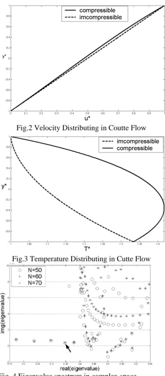
Methods for the solution of linear stability for compressible boundary layers are developed. Both the global and local methods for stability analysis are used. Both methods are use in solution of Coutte shear flow and the results are analysis and compare.

Some well-known conclusions of Coutte flow are proved by these methods again.

Introduction

The transition to turbulence of the boundary plays an important role in airfoil design. The linear stability analysis of a typical fluid flow is the general tools in flow stability analysis. Transition to turbulence in a boundary layer is a nonlinear process, but the way in which nonlinearity develops depends on the linear behavior of initially small disturbance. For the incompressible flow and used the parallel-flow approximation, the solution of boundary flow stability is leaded to the definition of Orr-Sommerfeld eigenvalue problem. In incompressible parallel flow, the Squire theory is used to translating three- dimension stability problem into two-dimension problem.

In compressible boundary flow, the O-S equation is inapplicable. The disturbance terms aren’t only velocity and density, but also temperature, viscosity, thermal conductivity and specific heat. And the Squire theory doesn’t adapt to compressible flow. The parabolized stability equations (PSE) approach is more accurate and consistent than the classical O-S theory. Using finite-difference discretization, the differential equations in PSE are reduced to linear algebraic equations. The global eigenvalues can be obtained by solving the characteristic determinant of a generalized eigenvalue problem. QR algorithm is used to compute all the eigenvalues. The number of solutions is relative to number of grid points, and many of “spurious” eigenvalues appear for grid points.

A “spurious” eigenvalue is one which is not an eigenvalue of the differential operator. When filtering out these “spurious” eigenvalues, the global problem is solved. If a guess of the eigenvalues is available, then the eigenvalue may be purified by a local eigenvalue search procedure involving matrix inversion and Neton iteration. ^[1][2]

This paper develops a global method of solution to the compressible boundary flow stability. The method exploits the tridiagonal structure associated with a finite-difference representation of the operator

involved, to automatically filter out spurious eigenvalues and calculate the non-spurious eigenvectors. ^[3]The unstable one of all true eigenvalues is chose, and is picked as the guess value of local method. The discretization which is used in local method is more accurate than that in global method. Matrix inversion and Neton iteration are used to solution local eigenvalue, and to compute the corresponding eigenvector. ^[4][5]

Equation

Compressible Linear Stability Equations

The Navier-Stokes equations governing the flow of a viscous compressible ideal gas are

( v) 0 t

ρ ρ

∂ + ∇ =

∂ (1)

( ) ( ^{i j}) _ij

j j i

v v

v v v p v

t x x x

ρ⎡⎢⎣∂∂ + ∇ ⎤⎥⎦= −∇ +∂∂ ⎡⎢⎢⎣μ ∂∂ +∂∂ +δ λ∇ ⎤⎥⎥⎦

(2)

( ) ( ) ( )

p

T p

c v T v p k T

t t

ρ ^⎡⎢⎣^∂∂ + ∇ ^{⎤ ⎡}⎥ ⎢⎦ ⎣= ^∂∂ + ∇ ^⎤⎥⎦+ ∇ ∇ + Φ

(3)

p=ρRT (4) Where ρ is the density, p the pressure, v the velocity vector, T edge temperature, μ the first coefficient of viscosity, λ the second coefficient of viscosity, c_p the specific heat, k the thermal conductivity x₁ , x₂ x₃ is the three diction of Cattesian coordinates. The viscous dissipation Φ is given as

( ^j) ( )

i i

ij

j j i

u u u

x ^⎧μ x ^∂x δ λ v ^⎫

∂ ⎪ ∂ ⎪

Φ =∂ ⎨⎪⎩ ∂ +∂ + ∇ ⎬⎪⎭

(5)

In this case we use dimensionless quantities,

*_{j j}/

x =x l , t^*=tu_e/l, v^*=v u/ _e, T^*=T T/ _e,

* / _e

ρ =ρ ρ , p^* = p/(ρ_eu_e²) , μ^* =μ μ/ _e ,

* / _e

k =k k , c^*_p =c_p/c_pe, λ^*=λ λ/ _e

where l is reference length, l u/ _e time, u_e the mainstream edge velocity, ρ_e edge density, T_e edge temperature, μ_e edge viscosity, k_e edge thermal conductivity, c_pe edge specific heat, λ_e edge the second coefficient of viscosity. The variable with superscript “*” is the nondimensional.

We use Cattesion coordinates x^*, y^*, z^*, where x^*

is the streamwise direction, y^* the spanwise direction

and z^* is normal to the solid boundary. And the victor correspondence of three diction are u^*, v^*,

w*. The nondimensional Navier-Stokes equations is

* * * * * * *

* * * *

( ) ( ) ( )

u v w 0

t x y z

ρ ρ ρ ρ

∂ +∂ +∂ +∂ =

∂ ∂ ∂ ∂ (6)

* * 1

* 2 * *

* * Re * * 0

Du p u

l V

Dt x x x

ρ = −^∂ + ^⎧⎪⎨ ^{∂ ⎛}⎜ μ ^∂ + λ ∇ ^⎞⎟+

∂ ⎪⎩∂ ⎝ ∂ ⎠

* * * *

* *

* * * * * *

u v w u

y y x z x z

μ μ ^⎫

⎡ ⎛ ⎞⎤ ⎡ ⎛ ⎞⎤

∂ ⎢⎢ ⎜⎜∂ +∂ ⎟⎟⎥⎥+ ∂ ⎢⎢ ⎜⎜∂ +∂ ⎟⎟⎥⎥⎪⎬

∂ ⎣ ⎝∂ ∂ ⎠⎦ ∂ ⎣ ⎝∂ ∂ ⎠⎦⎭⎪ (7)

* * 1

* 2 * *

* * Re * * 0

Dv p v

l V

Dt y y y

ρ = −^∂∂ + ^⎛⎜⎜⎝∂^{∂ ⎛}⎜⎜⎝ μ ∂^∂ + λ ∇ ^⎞⎟⎟⎠

* * * *

* *

* * * * * *

v u v w

x x y z z y

μ μ ⎫

⎡ ⎛ ⎞⎤ ⎡ ⎛ ⎞⎤

∂ ⎢ ⎜∂ ∂ ⎟⎥ ∂ ⎢ ⎜∂ ∂ ⎟⎥⎪ +∂ ⎢⎣ ⎜⎝∂ +∂ ⎟⎠⎥⎦+∂ ⎢⎣ ⎜⎝∂ +∂ ⎟⎠⎥⎦⎭⎬⎪

(8)

* *

* * *

* * * * 0

1 2

Re

Dv p v

l V

Dt y y y

ρ = −^∂∂ + ^⎧⎨⎩∂^{∂ ⎛}⎜⎝ μ ∂^∂ + λ∇ ^⎞⎟⎠

* * * *

* *

* * * * * *

v u v w

x ^⎡μ ^⎛ x y ^⎞⎤ z ^⎡μ ^⎛ z y ^⎞⎤⎫

∂ ∂ ∂ ∂ ∂ ∂ ⎪

+∂ ⎢⎣ ⎜⎝∂ +∂ ⎟⎠⎥⎦+∂ ⎢⎣ ⎜⎝∂ +∂ ⎟⎠ ⎪⎥⎦⎭⎬

(9)

* *

* * * * * * *

* *

1 ( )

Re Pr Re

p

DT Dp Ec

c Ec k T

Dt Dt

ρ = + ∇ ∇ + Φ (10)

( )

* * *

1

ECp T

γ = γ − ρ (11)

Where l₀ =λ μ_e/ _e is viscosity ratio,

2/( )

e pe e

Ec=u c T is Eckert number,

Pr=μ_ec_pe/k_e is Prandtl number, γ =c_p/c_v is specific heat ratio. In ideal gas, c^*_p =1. Where

* * *

* * * * *

* ( * *^j) 0 ( )

i i

ij

j j i

u u u

l v

x ^⎧μ x ^∂x δ λ ^⎫

∂ ⎪ ∂ ⎪

Φ =∂ ⎨⎪⎩ ∂ +∂ + ∇ ⎬⎪⎭

(12) The instantaneous nondimensional values can be represented as the sum of a mean and a fluctuation quantity,

u* = +U u′ , v^* = +V v′ , w^* =W +w′ ,

p*= +P p′ , T^* = +T T ′ , ρ^* = +ρ ρ′ ,

μ* = +μ μ′, λ^* = +λ λ′, k^* = +k k′

Substituting these into the nondimensional equation and dropping the mean quantities, yields the linearized perturbation equation

* * * *

( ) ( ) ( )

u u v v w w 0

t x y z

ρ′ ρ ′ ρ′ ρ ′ ρ′ ρ ′ ρ′

∂ +∂ + +∂ + +∂ + =

∂ ∂ ∂ ∂

(13)

( ) ( )

* * * * * * *

* * * *

1 2 2

0 0 0 0

* * * * *

R e

0 * 0 * * *

u u U u U u U

U u V v W w

t x x y y z z

U U U p

U V W

x y z x

U V W u

l l l l

x x y z x

v w u

l l

y z y y

ρ ρ

μ λ λ λ μ λ

λ λ μ

⎛∂ ′+ ∂ ′+ ′∂ + ∂ ′+ ′∂ + ∂ ′+ ′∂ ⎞

⎜∂ ∂ ∂ ∂ ∂ ∂ ∂ ⎟

⎝ ⎠

⎛ ∂ ∂ ∂ ⎞ ∂ ′

′

+ ⎜⎝ ∂ + ∂ + ∂ ⎟⎠= −∂ +

⎧ ∂ ⎡ ∂ ∂ ∂ ∂ ′

⎪ ⎢ ′+ ′ + ′ + ′ + +

⎨∂ ⎢ ∂ ∂ ∂ ∂

⎪ ⎣

⎩

′ ′⎤ ′ ′

∂ ∂ ⎥ ∂ ∂ ∂

+ + + +

∂ ∂ ⎥⎦ ∂ ∂ * * *

v U V

x y x

⎡ ⎛ ⎞ μ ⎛∂ ∂ ⎞⎤

⎢ ⎜⎜ ⎟⎟+ ′⎜⎜ + ⎟⎟⎥

⎢ ⎝ ∂ ⎠ ⎝∂ ∂ ⎠⎥

⎣ ⎦

W U

* * * * *

w u

z x z x z

μ μ ^⎫

⎡ ⎛ ′ ′⎞ ⎛ ⎞⎤

∂ ∂ ∂ ′ ∂ ∂ ⎪

+ ⎢ ⎜ + ⎟+ ⎜ + ⎟ ⎬⎥

⎢ ⎥

∂ ⎣ ⎝∂ ∂ ⎠ ⎝∂ ∂ ⎠ ⎪⎦⎭

(14)

( )

* * * * * * *

* * * *

1

0

* * * * * * *

R e

2 0 * 0

v v V v V v V

U u V v W w

t x x y y z z

V V V p

U V W

x y z y

u v U V U

l

x y x y x y x

l V l

y ρ

ρ

μ μ λ

μ λ λ

⎛∂ ′+ ∂ ′+ ′∂ + ∂ ′+ ′∂ + ∂ ′+ ′∂ ⎞

⎜∂ ∂ ∂ ∂ ∂ ∂ ∂ ⎟

⎝ ⎠

⎛ ∂ ∂ ∂ ⎞ ∂ ′

′

+ ⎜⎝ ∂ + ∂ + ∂ ⎟⎠= −∂ +

⎧ ∂ ⎡ ⎛ ∂ ′ ∂ ′⎞ ⎛∂ ∂ ⎞⎤ ∂ ⎡ ∂

⎪ ⎢ ⎜ + ⎟+ ′⎜ + ⎟⎥+ ′

⎨∂ ⎢ ⎜∂ ∂ ⎟ ⎜∂ ∂ ⎟⎥ ∂ ⎢⎣ ∂

⎪ ⎣ ⎝ ⎠ ⎝ ⎠⎦

⎩

∂ ∂

′ ′ ′

+ + +

∂ ^W_* ^l₀ ^u_* (^{2 l}₀ ) ^v_*

z x y

λ ^{∂ ′} μ λ ^{∂ ′}

+ + + +

∂ ∂ ∂

V W

0 * * * * * *

w v w

l

z z z y z y

λ∂∂ ′⎤⎥⎦+∂∂ ⎡⎢⎢⎣μ⎛⎜⎜⎝∂∂ ′+∂∂ ′⎞⎟⎟⎠+μ′⎛⎜⎜⎝∂∂ +∂∂ ⎞⎟⎟⎠⎤⎥⎥⎦⎭⎫⎪⎬⎪ (15)

* * * * * * *

* * * *

1 W U

* * * * * * * *

R e

*

w w W w W w W

U u V v W w

t x x y y z z

W W W p

U V W

x y z z

w u w v

x x z x z y y z

W y ρ

ρ

μ μ μ

μ

⎛∂ ′+ ∂ ′+ ′∂ + ∂ ′+ ′∂ + ∂ ′+ ′∂ ⎞

⎜∂ ∂ ∂ ∂ ∂ ∂ ∂ ⎟

⎝ ⎠

⎛ ∂ ∂ ∂ ⎞ ∂ ′

+ ′⎜⎝ ∂ + ∂ + ∂ ⎟⎠= −∂ +

⎡ ⎛ ⎞

⎧ ∂ ⎡ ⎛∂ ′ ∂ ′⎞ ⎛∂ ∂ ⎞⎤ ∂ ∂ ′ ∂ ′

⎪ ⎢ ⎜ + ⎟+ ′⎜ + ⎟⎥+ ⎢ ⎜ + ⎟

⎨∂ ⎢ ⎝∂ ∂ ⎠ ⎝∂ ∂ ⎠⎥ ∂ ⎢ ⎜∂ ∂ ⎟

⎪ ⎣ ⎦

⎩ ⎣ ⎝ ⎠

∂ ∂

+ ′ +

∂ * * 0 * 0 * (² 0 ) *

V U V W

l l l

z z x y z

λ λ μ λ

⎛ ⎞⎤⎥ ∂ ⎡ ′∂ ′∂ ′ ′ ∂

⎜ ⎟ + ⎢ + + +

⎜ ∂ ⎟ ⎥ ∂ ⎢ ∂ ∂ ∂

⎝ ⎠⎦ ⎣

(² )

0 * 0 * 0 *

u v w

l l l

x y z

λ^{∂ ′} λ ^{∂ ′} μ λ ^{∂ ′⎤⎫⎪}

+ + + + ⎥⎬

∂ ∂ ∂ ⎦⎪⎭

(16)

* * * * * * * * * *

* * * * * * * * * *

T T T T T T T T T T

U u V v W w U V W

t x x y y z z x y z

p p p p p p p p p p

Ec U u V v W w Ec U V W

t x x y y z z x y z

ρ ρ

ρ ρ

⎡∂ ′+ ∂ ′+′∂ + ∂ ′+′∂ + ∂ ′+ ′∂ ⎤+ ′⎛⎜ ∂ + ∂ + ∂ ⎞⎟=

⎢∂ ∂ ∂ ∂ ∂ ∂ ∂ ⎥ ∂ ∂ ∂

⎣ ⎦ ⎝ ⎠

⎡∂′+ ∂′+ ′∂ + ∂′+′∂ + ∂′+ ′∂ ⎤+ ′⎛⎜ ∂ + ∂ + ∂ ⎞⎟

⎢∂ ∂ ∂ ∂ ∂ ∂ ∂ ⎥ ∂ ∂ ∂

⎣ ⎦ ⎝ ⎠

* * * * * * * * *

1 Re Pr

T T T T T T

k k k k k k

x x x y y y z z z

⎡ ∂ ⎛ ∂ ′ ′∂ ⎞ ∂ ⎛ ∂ ′ ′∂ ⎞ ∂ ⎛ ∂ ′ ′∂ ⎞⎤ + ⎢⎢⎣∂ ⎜⎝ ∂ + ∂ ⎟⎠+∂ ⎜⎝ ∂ + ∂ ⎟⎠+∂ ⎜⎝ ∂ + ∂ ⎟⎠⎥⎥⎦

{ 4 * * * * * * 2 * * * *

Re

Ec U u V v W w V U v u

x x y y z z x y x y

μ^{⎡ ⎛∂ ∂ ′ ∂ ∂′ ∂ ∂ ′⎞ ⎛∂ ∂ ⎞⎛∂′ ∂′⎞} + ⎢ ⎜⎢⎣ ⎝∂ ∂ +∂ ∂ +∂ ∂ ⎟⎠+ ⎜⎝∂ +∂ ⎟⎜⎠⎝∂ +∂ ⎟⎠

* * * * * * * *

2 W V w v 2 U W u w

y z y z z x z x

⎛∂ ∂ ⎞⎛∂ ′ ∂ ′⎞ ⎛∂ ∂ ⎞⎛∂ ′ ∂ ′⎞⎤ + ⎜⎝∂ +∂ ⎟⎠⎜⎝∂ +∂ ⎟⎠+ ⎜⎝∂ +∂ ⎟⎠⎜⎝∂ +∂ ⎟⎠⎥⎥⎦

2 2 2

0 * * * * * * * * *

2 U V W u v w 2 U 2 V 2 W

l x y z x y z x y z

λ ^{⎛∂ ∂ ∂ ⎞⎛∂′ ∂′ ∂′⎞} μ′⎢^{⎡ ⎛∂ ⎞ ⎛∂ ⎞ ⎛∂ ⎞} + ⎜⎝∂ +∂ +∂ ⎟⎠⎜⎝∂ +∂ +∂ ⎟⎠+ ⎢⎣ ⎜⎝∂ ⎟⎠ + ⎜⎝∂ ⎟⎠+ ⎜⎝∂ ⎟⎠

2 2 2 2

* * * * * * 0 * * *

V U W V U W U V W

l

x y y z z x ⎤ λ x y z ⎫

⎛∂ ∂ ⎞ ⎛∂ ∂ ⎞ ⎛∂ ∂ ⎞⎥ ′ ⎛∂ ∂ ∂ ⎞⎪

+⎜⎝∂ +∂ ⎟⎠+⎜⎝∂ +∂ ⎟⎠ +⎜⎝∂ +∂ ⎟⎠⎥⎦+ ⎜⎝∂ +∂ +∂ ⎟⎠ ⎪⎬⎭

（ 17 ）

( ¹)( )

ECp T T

γ ′= γ − ρ ′+ρ′ (18)

Using Stokes assumption

/ const 2 / 3

λ μ= = − (19)

So

* *

λ =μ , l₀ = −2 / 3 (20) Assumed μ μ= ( )T , λ λ= ( )T , k=k T( ), they are all function of temperature. So we can write

d T dT

μ′= μ ′, ^d _T dT

λ′= λ ′, d k

k T

dT

′= ′ (21) n boundary layer assumption

* 0

p y

∂ =

∂ ^,

( *)

U =U y , W =W y( ^*), T =T y( ^*),

(y*)

ρ ρ= , V =0 (22)

So the mean equation of state is

1=ρT (23)

So