Simplified Method for the Determination of Cumulative Landslide Displacement in the Event of an Earthquake
using “Slide Block” Type Analyses
지진발생시 Slide Block형 분석을 이용한 누적 산사태 변위 결정 단순법
배 윤 신1* Bae, Yoon-Shin
ABSTRACT
Earthquake induced landslides have caused tens of thousands of deaths and billions of dollars of damage during the last century alone. Determining the potential seismic hazard presented by statically stable slopes is essential for the evaluation of substantial landslide movement during an earthquake. Newmark’s method for estimating landslide displacement under dynamic loading was presented and applied to two case studies. A simplified energy-based method was then be developed to estimate the Newmark’s displacement.
요 지
지진을 수반한 산사태는 지난 십년동안 수만명의 사상자와 수십억불의 재난피해를 초래해 왔다. 정역학적으로 안정된 경사로 표현되는 잠재적 지진 위험요소를 결정하는 것은 지진이 발생하는 동안 중요한 움직임을 평가하는데 필수적이다. 동적 하중에
서의 산사태 움직임을 추정하기 위한 Newmark 방법이 소개되고 두 사례에 적용되었다. 그리고 에너지에 근거한 간략법이
Newmark의 변위를 추정하기 위하여 개발되었다.
Keywords : Landslides, Seismic hazard, Earthquake, Newmark’s method 한국토목섬유학회논문집 제8권 1호 2009년 3월 pp. 1 ∼ 10
J. Korean Geosynthetics Society Vol.8 No.1 March. 2009 pp. 1 ~ 10
1* 정회원, 공학박사, 한국해양연구원 연안개발에너지 연구부 연수연구원 (Member, Korea Ocean Research & Development Institute, E-mail: [email protected])
1. INTRODUCTION
The bearing capacity improvement of soils provides the possibility for the use of geosynthetics in reinforcing soils. The performance of these geosynthetics has been found to be dependent on a number of variables. Some of the more commonly identified include: 1) the original stress in the geotextile 2) the number of layers to be used 3) the depth geosynthetics are used over and 4) the type of geosynthetic. Additional failure mechanisms such as failure above the upper geotextile, insufficient embedment length, tensile failure of the geotextile and excessive
creep must also be considered when designing for bearing capacity improvement.
However, dynamic loading caused by an earthquake not only destroys the structures using geosynthetics for stabilization and reinforcement, it also weakens the strength of the soil by remolding the soil fabric and increasing pore pressures (Herzog and Nilsson, 1996).
The types of failures include landslides, liquefaction events, rock falls, slumps, and avalanches, In many earthquakes, the landslides cause the most damage because they can overrun people and structures, block roads, and sever lifelines such as water pipes, power
lines, or gas mains. Roads blocked by landslides can also isolate communities from much needed emergency help or relief (Wilson and Keefer, 1985). A technique to predict the displacement of landslides during earthquake is essential to determine those slopes that are in the most need of stabilization efforts. An introduction to the simplest approach to landslide stability, the pseudostatic analysis, is discussed. A more in-depth look at the Newmark sliding block method will follow. Finally, a new simplified technique to estimate the Newmark displacement based on the energy and intensity of a given earthquake ground motion will be developed through the analysis of 20 different earthquake records. Conclusions will be drawn as to the validity of the aforementioned
“simple energy” and its accuracy in predicting landslide displacements.
1.1 Pseudostatic Analysis
The simplest approach to analyzing the seismic performance of a slope is modeled as a rigid block. The earthquake acceleration acting on the mass of a potential landslide is treated as a permanent static body force in a limit equilibrium (factor-of-safety) analysis (Jibson, 1993). The acceleration required to lower the factor of safety to 1.0 is called the yield, or critical, acceleration (ac). An acceleration that is greater than the critical acceleration will lower the factor of safety below 1.0 and the slope will fail. The simplicity of the procedure lies in the fact that no more information is needed than is what is reduced for a static factor of safety analysis. The pseudostatic factor of safety of a slope (FS) can be expressed as (Kramer, 1996):
β β
φ β β
cos sin
) (
tan ] sin cos
) [(
h V
h V
ab
F F
W
F F
W FS cl
+
−
−
−
= + (1)
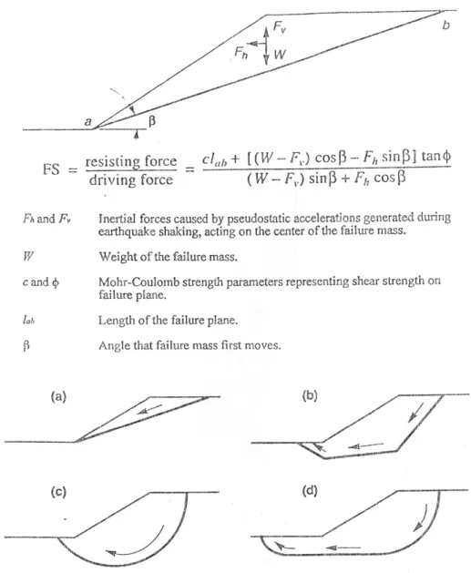
where c and φ are the Mohr-Coulomb strength parameters that give the soil strength on the failure plane, lab is the length of the failure plane, W is the weight of the soil mass, β is the angle of inclination of the slope, and Fv
and Fh are the vertical and horizontal components,
respectively, of the pseudostatic forces induced by the earthquake. These variables are more clearly demonstrated in Fig. 1.
The relative simplicity of the pseudostatic approach does not come without some shortcomings. The pseudostatic analysis is useful for predicting critical accelerations and peak ground accelerations (PGA) below which no ground movement will occur. However, in the instance that the critical acceleration of PGA is exceeded, the pseudostatic approach tells nothing about the subsequent displacement of the slope (Jibson, 1993). Modeling the complex motions of an earthquake as a single, constant, unidirec- tional acceleration is oversimplified. Terzaghi (1950) stated that “the concept it conveys of earthquake efforts on slope is very inaccurate, to say the least,” and a factor of safety greater than 1.0 does not guarantee that a slope is stable. Case studies where the soils have the ability to build up large excess pore pressures and show more than 15% degradation of strength during an earthquake have failed with pseudostatic factors of safety greater than 1.0 (Kramer, 1996).
1.2 The Newmark Sliding Block Analysis The Newmark sliding block analysis is a good alternative to the simplistic pseudostatic methods and the complex finite element analyses. Newmark’s method models a landslide as a rigid-plastic friction block having critical acceleration (ac) above which the driving force will exceed the frictional resistance of the slope and sliding will commence. The 1st step is to determine the factor of safety (FS) and the 2nd step in the Newmark analysis is to obtain this critical acceleration. It is given by (Jibson, 1993):
ac=(FS-1)g*sinα (2)
where ac is the critical acceleration with unit of g, FS is the static factor of safety of the selected slope, and α is the angle (thrust angle) from the horizontal that the center of mass of the potential land slide mass first moves. Thus, the critical acceleration is easily obtained given the static
Fig. 1. Explanation of Eq. (1) for determining factor of safety, and common failure surface geometries for sliding-block type landslides: (a) planar-similar to the 8th avenue analyzed in this paper; (b) multiplanar; (c) circular-similar to Anderson lake reviewed in this paper; (d) noncircular (After Kramer, 1996)
factor of safety and the thrust angle. The static factor of safety can be determined through a variety of procedures including method of slices, infinite slope, moment equilibrium, chart solutions, and appropriate computer programs such as STABL.
The most difficult part in conducting the Newmark analysis is selecting an input ground motion that is appropriate for the landslide of interest. Most studies use a combination of two approaches: (a) scaling acceleration time histories from actual earthquakes to design PGA values and (b) using singular or multiple cycles of generic (sinusoidal, triangular, or rectangular) motions (Jibson, 1993). Unfortunately, each approach has its strengths and
weaknesses and must be left up to the engineering judgment of the individual to make the most appropriate decision.
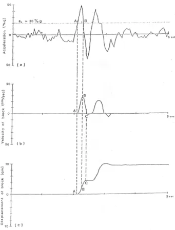
Now that the critical acceleration and acceleration time history have been obtained, the prediction of block displacement can be calculated. The block will move relative to the firm base at each instant the acceleration time history exceeds the critical acceleration and is illustrated in Fig. 2. The block will accelerate (ar) at a value equal to the difference of the maximum ground acceleration and the critical acceleration. The acceleration record is integrated twice over each period in which acceleration exceeds ac to calculate the relative velocity
Fig. 2. Acceleration of the sliding block translates to movement (Wilson and Keefer, 1985)
(vr) and displacement (dr) (Kramer, 1996).
∫
=
t
t r
r t a t dt
v
0
) ( )
( (3)
∫
=t
t r
r t v t dt
d
0
) ( )
( (4)
The Newmark method also does not directly account for continued movement from momentum after ar<0. One would not expect the landslide mass stop moving immediately after acceleration ceases, just as a car does not stop immediately after the throttle is reduced. The simplest and most widely used method is to double the Newmark displacement, which is essentially assuming the block decelerates at the same rate as it accelerates (Jibson, 1993). Another approach developed by Byrne et al. (1992) uses an energy principle analysis based on Newmark’s model to estimate displacements. Their method centers on the work-energy theorem where the external work minus the internal work must be equal to the change in kinetic energy of the system. Therefore, for
a single velocity pulse, the displacement is given by (Byrne et al., 1992):
gN d V
2 2
/
=1 (5)
where g is the acceleration due to gravity, N is the critical acceleration, and V is the magnitude of the velocity pulse.
The potential increase or decrease in soil strength once the soil is subjected to dynamic loading is another issue that not directly addressed in the Newmark analysis. The static factor of safety is assumed to be constant during the entire earthquake. However, in brittle, strain-softening, or liquefiable material, the shear strength decreases with increasing shear strength with increasing rate of shear (Vessely and Cornforth, 1998). In the former, an under- estimate of the displacement and in the latter, an overestimate of the displacement will occur. With this being said, most analyses are still conducted using constant factors of safety to simplify the process.
2. CASE STUDIES
The two case studies that will be analyzed show the Newmark analysis procedure and the accuracy of the method when compared to the actual measured displace- ments of the slides. Both slides are the result of seismic events where the ground motions were recorded at nearby stations.
2.1 Lake Anderson Slide, California
The lake Anderson slide was caused by the Coyote Lake, California earthquake of August 6, 1979 and had a Richter magnitude (ML) of 5.9. The earthquake was triggered by movement along the Calaveras fault, which is a right-lateral strike-slip fault located in central California and is part of the San Andreas Fault zone (Fig. 3, Armstrong, 1979). The resulting landslide had a fissure up to 21 mm wide (Wilson and Keefer, 1983).
The Newmark analysis of the slide was performed by Wilson and Keefer (1983) using two nearby rock motion
Fig. 3. Location of the 8th avenue and Anderson Lake slides and strong-motion stations used in the analyses records. An ac of 0.22 g was used on a friction angle
(φ) of 25° and a cohesion of 14.36 kPa. The first strong motion record, Coyote Creek (250°), had a maximum peak acceleration of 0.23 g. The calculated displacement of 0.12 mm was significantly less than the measured displacement. A second trial using the N50° E component of the Gilory #6 record was performed. With an ac of 0.42 g, it nearly doubled that of the Coyote Creek record.
The calculated Newmark displacement was 27 mm and much closer to the actual displacement of 21 mm that was measured in the field (Wilson and Keefer, 1983).
There were a variety of explanations given for the
differences between the calculated Newmark displacement and the field measurements. The first had to do with topographical effects. The Coyote Creek station lies at the bottom of a valley and the Anderson Lake slide occurred at the top of a ridge. Ridge tops may amplify accelerations up to 1.5 times whereas valleys may deamplify by as much as 0.75 times (Wilson and Keefer, 1983). Gilory
#6 was, in fact, near a ridge top. A second explanation was that the Coyote Lake earthquake exhibited a surface rupture along the Calveras fault that was nearly twice as long as expected. The fact that it ruptured to the surface is unexpected (Armstrong, 1979).
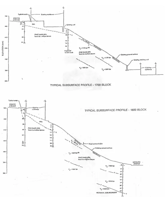
Fig. 4. Slope profiles (Herzog and Nilsson, 1996) 2.2 Eighth Avenue Slide, San Francisco
The Eighth Avenue slide was caused by the Loma Prieta earthquake (Ms=7.1) which occurred on October 17, 1989. The earthquake was a result of a ±45 km rupture of the San Andreas fault northeast of Santa Cruz, California (Herzog and Nilson, 1996). The Eighth Avenue site has since been stabilized with a combination of drilled soldier piles and permanent tiebacks (Shields and Rollo, 1990). A significant amount of soil testing went into the design of the retaining system and soil properties and slope profiles are readily available. Using this data along with acceleration records from nearby strong motion stations, Herzog and Nilsson (1996)
conducted a Newmark analysis in a case study. Fig. 3 contains a local map for the slide.
Fig. 4 shows the slop profile for the 1700 and 1800 blocks of Eighth Avenue, respectively (Shields and Rollo, 1990). The hillside slope downward 32° to 35° from Eighth Avenue to Seventh Avenue. The slide occurred in a dune sand deposit which is up to 45.7m thick in areas around San Francisco. The relative uniform soil profile allowed for a simple infinite slope analysis to obtain the static factor of safety. The static factor of safety for a cohesionless soil is given as:
β φ tan
= tan
FS (6)
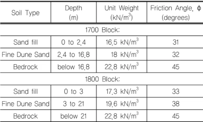
Table 1. Estimated soil parameters Soil Type Depth
(m)
Unit Weight (kN/m3)
Friction Angle, φ (degrees) 1700 Block:
Sand fill 0 to 2.4 16.5 kN/m3 31 Fine Dune Sand 2.4 to 16.8 18 kN/m3 32 Bedrock below 16.8 22.8 kN/m3 45
1800 Block:
Sand fill 0 to 3 17.3 kN/m3 33 Fine Dune Sand 3 to 21 19.6 kN/m3 38 Bedrock below 21 22.8 kN/m3 45
Table 2. Summary of results considering positive and negative critical acclerations
Motion Recorded Location Maximum Velocity (cm/sec)
Permanent Displacement (cm) Positive accelerations
Cliff House Station
1700 Block 13.7 6.3
1800 Block 26.3 23.5
Diamond Hts.
Station
1700 Block 2.5 1.4
1800 Block 13.4 10.3
Negative accelerations Cliff House
Station
1700 Block 12.4 4.6
1800 Block 20.4 19.1
Diamond Hts.
Station
1700 Block 8.2 1.8
1800 Block 13.2 8.1
where φ is the friction angle of the soil and β is the angle of inclination of the slope. The estimated soil parameters used by Herzog and Nilsson (1996) are given in Table 1.
The resulting factors of safety were very close to 1.0. A second static factor of safety was performed using the STABL/G computer program and factor of safety were 1.074 and 1.025 for the 1700 and 1800 blocks, respectively.
These factors of safety were used in conjunction with Eq, (2) to determine the critical accelerations. They were 0.039 g and 0.013 g for the 1700 and 1800 blocks, respectively (Herzog and Nilsson, 1996). Very small magnitudes of shaking would be sufficient to initiate movement in either case.
Two rock motion records were used in the Newmark displacement analysis. The first was the Diamond Height Station located approximately 73 km from the rupture zone, and the second was Cliff House Station located about 80 km from the rupture zone. Both stations were within 7 km of the Eighth Avenue slide (Herzog and Nilsson, 1996). The records are typically given in an 8 column, 250 row format and must be converted into 1 column in chorological order for a spreadsheet analysis. The simplest way to accomplish this transformation is to open the file in Microsoft Word and replace all of the tab commands with return commands. Herzog and Nilsson (1996) used a FORTRAN program to do this conversion.
A spreadsheet can be developed to perform the necessary double integration of the acceleration record to obtain the displacement of the landslide. Only those acceleration values that exceed the critical acceleration (ac) are integrated. Positive change in velocity are
recorded where a> ac and negative changes where a< ac. Negative changes in velocity, (deceleration) were incrementally added until the cumulative velocity returned to zero which signifies the block stopped moving. Positive values of velocity showed where, in time, the block was moving.
This velocity record is then integrated to obtain the permanent displacement of the slide. Each incremental displacement is summed to calculate the cumulative displacement (Herzog and Nilsson, 1996). The following
“If, then” formulas were used in a Microsoft Excel spreadsheet to calculate the change in velocity (V), velocity (V), and displacement (d):
V=(a-ac)*dt (7)
Vn=IF(Vn-1+Vn<0,0,IF(Vn-1>0,(Vn-1+Vn),
IF(Vn>0,(Vn-1+Vn)))) (8)
dn=dn-1+(Vn*dt) (9)
In their analysis, Herzog and Nilsson (1996) used the negative values of the acceleration records when the peak accelerations were negative. The decision was made to obtain conservative displacements. A table of their results is as follows:
Measured displacements were as much as 15.25 cm horizontal and 10 cm of vertical movement (Shields and Rollo, 1990). Herzog and Nilsson (1996) concluded that
“the estimates using the Newmark method were low for the 1700 block (1.4 to 6.3 cm), but reasonably accurate for the 1800 block (10.3 to 23.5 cm).”
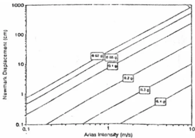
Fig. 5. Newmark displacement as a function of Arias intensity for several values of critical acceleration (Jibson, 1993) 2.3 Development of Simplified Method to
Determine Newmark Displacement
The previous discussion has centered on the procedure by which the displacement of a landslide can be calculated using the Newmark analysis. The technique has shown to give relatively accurate results given an appropriate rock motion record, reliable soil parameters, and slope geometry for the slide mass in question.
However, both case studies have proven that Newmark method is very time consuming if a computer spreadsheet with an integration program is not readily available. One might argue that a simplified technique could be developed where the whole spreadsheet analysis is bypassed, and an estimate of the Newmark displacement could be made faster, easier, and within one order of magnitude of the actual landslide displacement.
A concept developed by Arias (1970) called the Arias intensity is a comprehensive and quantitative measure of total shaking intensity. Arias intensity is given by the equation:
∫
= g a t dt
Ia π/2 [ ()]2 (10)
where Ia is the Arias intensity (units of velocity), and a(t) is the ground acceleration as a function of time, The Arias intensity is essentially a summation of the area bounded by the x-axis and the acceleration time history curve squared for a duration of the entire record.
The duration is the Dobry duration as specified in Dobry (1978). A figure was developed based on 11 different strong motion records that plotted Newmark displacement as a function of Arias intensity for different values of critical acceleration. Jibson (1993) developed this method as a simplified version of the Newmark analysis, but it is still necessary to perform an integration of the acceleration record to obtain the Arias intensity, and in turn, use Fig. 5 to get the Newmark displacement.
The figure could easily yield a range of Newmark displacements that are an order of magnitude different from each other if the critical acceleration is not precisely known.
2.4 Simple Energy
An even simpler approach than the Arias intensity method developed by Jibson would be to define new
“simple energy” where, given an acceleration time history and a critical acceleration, one could quickly and easily correlate the “simple energy” to the Newmark displacement through the use of a figure. The method would not require a computer program and could potentially be performed in a matter of minutes.
The simple energy is basically a quick estimate of the area above the critical acceleration and below the acceleration time history. The duration over which this area calculation is made starts at the first instant in time that a>ac and ends at the last instant in time a<ac. The simple energy (SE) has the units of velocity and is calculated with the following equation.
SE=[Duration]*1/3(amax-ac)g (11) where amax is the maximum acceleration in the strong motion record, ac is the critical acceleration, and g is the acceleration due to gravity (cm/sec2). The 1/3 factor is included to account for the fact that the acceleration is not at a maximum throughout the defined duration and yields a more accurate estimate of the simple energy.
Acceleration time histories are variable in intensity, maximum acceleration, and duration. Many strong motion records are not as “uniform” and may has numerous peaks where the critical acceleration is exceeded but are
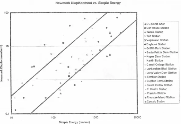
Fig. 6. Newmark displacement plotted as a function of simple energy separated by many seconds. These “non-uniform” accele-
ration records will exhibit simple energy values that are extraordinarily high for relatively small Newmark displace- ments. The simple energy method is highly dependent on the duration previously defined and the practitioner is at the mercy of the particular acceleration time history that he/she selects.
Now that the simple energy has been calculated, the Newmark displacement can be obtained by scaling the value off of Fig. 6. Fig. 6 shows the Newmark displace- ment plotted as a function of the simple energy. Calculating the Newmark displacement and simple energy at various critical accelerations over a span of 20 different accele- ration time histories developed the plot. The data points for each acceleration record were essentially linear when plotted on log-log axes. However, the slopes of the lines were different for each which was a result of the varying plots of each strong motion record. Two parallel, linear lines drawn in the plot to provide a range of Newmark displacements for each values of the simple energy, The displacement could vary by an order of magnitude which is consistent with the plot given in Fig. 5 (Jibson, 1993).
The two lines encompass 70% of the data that was
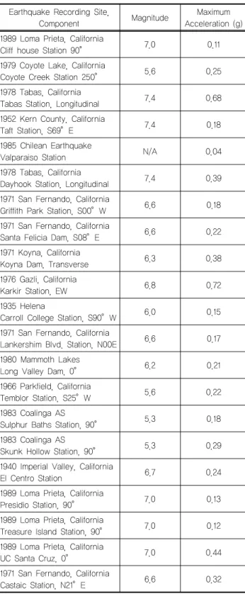
collected. Table 3 summarizes the strong motion records that were selected for the analysis.
At the simple energy of 180 cm.sec, Fig. 6 would suggest a maximum Newmark displacement of about 8 cm. The spreadsheet solution yields a displacement of 12.5 cm and the actual measured displacement on the Eighth Avenue slide was about 15 cm. The simple energy method of calculating the Newmark displacement was well within the one order of magnitude error. Note that this simple energy method for determining the Newmark displacement was developed for parishioners who need quick estimates of potential accuracy to determine if a more rigorous analysis is warranted in the future for the particular case in question.
3. CONCLUSION
The Newmark sliding block analysis is a good method to characterize seismic slope response (Jibson, 1993). It is a practical alternative to the simplistic pseudostatic method and the complex finite element analyses. The new simplified energy presented here provides an easy way to obtain the Newmark displacement if the critical acceleration
Table 3. Strong‐motion records selected for analysis Earthquake Recording Site,
Component Magnitude Maximum
Acceleration (g) 1989 Loma Prieta, California
Cliff house Station 90° 7.0 0.11
1979 Coyote Lake, California
Coyote Creek Station 250° 5.6 0.25 1978 Tabas, California
Tabas Station, Longitudinal 7.4 0.68 1952 Kern County, California
Taft Station, S69°E 7.4 0.18
1985 Chilean Earthquake
Valparaiso Station N/A 0.04
1978 Tabas, California
Dayhook Station, Longitudinal 7.4 0.39 1971 San Fernando, California
Griffith Park Station, S00°W 6.6 0.18 1971 San Fernando, California
Santa Felicia Dam, S08°E 6.6 0.22
1971 Koyna, California
Koyna Dam, Transverse 6.3 0.38
1976 Gazli, California
Karkir Station, EW 6.8 0.72
1935 Helena
Carroll College Station, S90°W 6.0 0.15 1971 San Fernando, California
Lankershim Blvd. Station, N00E 6.6 0.17 1980 Mammoth Lakes
Long Valley Dam, 0° 6.2 0.21
1966 Parkfield, California
Temblor Station, S25°W 5.6 0.22
1983 Coalinga AS
Sulphur Baths Station, 90° 5.3 0.18 1983 Coalinga AS
Skunk Hollow Station, 90° 5.3 0.29 1940 Imperial Valley, California
El Centro Station 6.7 0.24
1989 Loma Prieta, California
Presidio Station, 90° 7.0 0.13
1989 Loma Prieta, California
Treasure Island Station, 90° 7.0 0.12 1989 Loma Prieta, California
UC Santa Cruz, 0° 7.0 0.44
1971 San Fernando, California
Castaic Station, N21°E 6.6 0.32
and representative acceleration time history can be obtained. The simple energy method, when applied to the Eighth Avenue case study, performed within the range of
error that can be expected with a more involved Newmark analysis procedure. The simple energy analysis is the procedure to consider when a more complicated, sophisticated, or expensive method is not practical.
REFERENCES
1. Arias, A., (1970), “A Measure of Earthquake Intensity,”
Seismic Design for Nuclear Power Plants, Massachusetts Institute of Technology Press, Cambridge, pp.438-483 2. Armstrong, C. F., (1979), “Cotote Lake Earthquake 6 August
1979,” California Geology 32, pp.248-251.
3. Dobry, R., I. M. Idriss, and E. Ng., (1978), “Duration Characteristics of Horizontal Components of Strong-Motion Earthquake Records,” Bulletin of the Seismological Society of America, Vol.68, No.5, pp.1487-1520.
4. Herzog, D. W., and Nilssom, M. K., (1996), Determining Cumulative Displacement of Landslides Using “Sliding-Block”
Type Analyses, Corvallis, Ore.
5. Jibson, R. W. (1993), “Predicting Earthquake-Induced Landslide Displacements Using Newmark’s Sliding Block Analysis,”
Transportation Research Record, No. 1411-Earthquake-Induced Ground Failure Hazards, Transportation Research Board, National Research Council, Washington, D.C., pp.9-17.
6. Kramer, S. L. (1996). Geotechnical Earthquake Engineering, Upper Saddle River, New Jersey: Prentice Hall.
7. Shields, C. S., and Rollo, F. L. (1990), Retaining Structure to Mitigate Seismic-Induced Movement of Steep Slope in Dune Sand. San Francisco: Treadwell and Rollo, Inc.
8. Terzaghi, K. (1950), “Mechanisms of landslides,” Engineering Geology (Berkeley) Volume, Geological Society of America.
9. Vessely, D. A., and Cornforth, D. H., (1998), “Estimating Seismic Displacements of Marginally Stable Landslides Using Newmark Approach,” Geotechnical Earthquake Engineering and Soil Dynamics III (Volume I), American Society of Civil Engineeris, pp.800-811.
10. Wilson, R. C., and Keefer, D. K. (1983), “Dynamic Analysis of a Slope Failure from the 6 August 1979 Coyote Lake, California, Earthquake,” Bulletin of the Seismological Society of America, Vol.73, No.3, pp.863-877.
11. Wilson, R. C., and Keefer, D. K. (1985), “Predicting Area Limits of Ear hake-Induced Landsliding, in Ziony, J. I., editor, Evaluating Earthquake Hazards in the Los Angeles Region: U. S. Geological Survey Professional Paper No.
1360, pp.317-345.
(논문접수일 2009. 2. 15, 심사완료일 2009. 2. 25)