韓國水資源學會論文集 第48卷 第12號 2015年 12月 pp. 1051~1064
선형계획법을 이용한 H 아리수 정수 센터 최적 취수량 결정
Determination of Optimal Hourly Water Intake Amount for H Arisu Purification Center using Linear Programming
이 철 수* / 이 강 원**
Lee, Chulsoo / Lee, Kangwon
...
Abstract
Currently, the H purification plant determines the hourly water intake amount based on operator experience and skill. Therefore, inevitably, there are deviations among operators. While meeting time- varying demand and maintaining the proper water level in the clean water reservoir, the methodology for minimizing electricity cost, when dealing with different electricity rate time zones, is a very complicated problem, which is beyond an operator’s capability. To solve this problem, a linear programming (LP) model is proposed, which can determine the optimal hourly water intake amount for minimizing the daily electricity cost. It is shown that an inaccurate estimate for the hourly water usage in the demand areas causes the water level constraint to be violated, which is the weak point of the proposed LP method. However, several examples with real-field data show that we can practically and safely solve this problem with safety margins. It is also shown that the safety margin method still works effectively whether the estimate is accurate or not. The operators need not attend the site at all times under the proposed LP method, and we can additionally expect reductions in labor costs.
Keywords : water purification plant, water intake station, linear programming, demand forecast
...
요 지
본 논문은 선형계획모형을 이용하여 H 아리수 정수 센터의 최적 취수량 결정 방법을 연구 하였다. 현재 H 아리수 센터에서는 관리자의 경험과 숙련도에 의지하여 취수량을 결정하고 있다. 그런데 매시 변하는 수요를 만족 시키면서 시간대 별로 요금이 서로 다른 전력의 사용을 최소화 하는 취수량 결정은 근무자들의 경험과 숙련도를 넘어서는 간단한 문제가 아니다. 따라서 수리적 기법 중 하나인 선형계획모형을 이용해 취수량을 결정하고, 비용 절감을 시도하였다. 본 연구에서 제안한 선형계획 모형은 수요예측치를 기본 입력자료로 사용하고 있는데 예측오차가 발생할 경우 정수지 높이 제한을 위반하는 경우가 발생한다. 이를 해결하기 위해서는 정확한 수요예측이 선행되어야 한다. 그러나 아무리 좋은 예측 기법을 사용하더라도 실수요와 오차는 있게 마련이고 이는 여전히 높이 제한의 제약을 만족 시키지 못하는 결과를 불러일으킨다.
따라서 예측오차를 수용 할 수 있는 안전 마진 상수를 이용한 대안을 제안하였다. 본 연구에서 제안한 선형 계획 모형을 통한 취수량 결정은 수위 모니터링을 위해 항시 작업자가 근무 할 필요가 없기 때문에 인건비 면에서도 많은 절약이 예측되어 총 비용 감축은 훨씬 더 많으리라 기대된다.
핵심용어 : 정수지, 취수장, 선형계획, 수요예측
...
* 서울과학기술대학교 글로벌융합산업공학과 연구원 (e-mail:[email protected])
Researcher, Department of Industrial and Information Systems Engineering, Seoul National University of Science&Technology, Seoul, Korea
** 교신저자, 서울과학기술대학교 글로벌융합산업공학과 교수 (e-mail:[email protected], Tel: 82-2-970-6476)
Corresponding Author, Professor, Department of Industrial and Information Systems Engineering, Seoul National University of Science&
Technology, Seoul, Korea
J. Korea Water Resour. Assoc.
Vol. 48, No. 12:1051-1064, December 2015 http://dx.doi.org/10.3741/JKWRA.2015.48.12.1051 pISSN 1226-6280 • eISSN 2287-6138
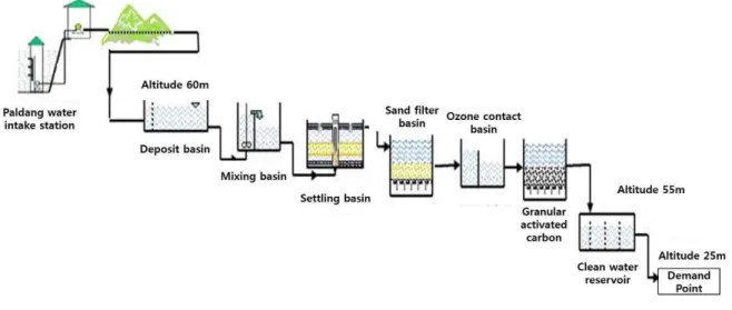
Fig. 1. Water Production Process in the Purification Plant
Deposit basin A
Deposit basin B
Main motor operative valve
Basin motor opertative A (M-102A)
Basin motor opertative B (M-102B) Paldang water
intake station
(M-101)
Fig. 2. Distributor in the Deposit Basin (H Arisu Purification Center, 2015) 1. Introduction
Seoul has six water purification plants to meet the water demand of city. The clean water production pro- cess in each purification plant is shown in Fig. 1.
The water intake station supplies water to the deposit basin, where water arrives first in the purification plant.
Chemicals are mixed into the water in the mixing basin, and alien substances settle in the settling basin. In the sand filter basin, the water is purified through sand, and alien substances are removed through ozone contact in the ozone contact basin. The granular activated carbon purifies the water with activated carbon and sand. The clean water reservoir temporarily stores the water before sending it to the demand point.
H purification plant is one of the six purification plants located at Seoul and supplies water to the areas of Kangdong, Songpa, and part of Hanam city [9]. Because H does not have its own water intake station, it receives water from the Paldang intake station. Paldng con- tinuously pumps water to meet the demand of H and many
other purification plants. H controls the amount of water it receives from Paldang with a motor-operated valve.
The distributor in the deposit basin is shown Fig. 2, where there are the main motor-operated valve (M-101) and 2 motor-operated valves (M-102A and M-102B).
Every hour, an operator determines the amount of water to receive from Paldang based on the hourly demand prediction, using his experience and skill. The operator supplies water to deposit basins A and B by properly controlling M-101A and M-101B, respectively. The water in the deposit basin arrives at the clean water reservoir after a six-hour production process as shown in Fig. 1.
Electric motors are used to move water between the locations shown in Fig. 1, and a significant amount of electricity is used to produce clean water. In order to minimize the electricity cost, more water should be produced when the electricity rate is lower and vice versa.
Currently, determining the hourly amount of water intake at H purification plant from the Paldang water intake station is largely based on an operator’s subjective
decision from their experience and skill. Therefore, inevitably, there are deviations among operators. Deter- mining the optimal amount of hourly water intake that can meet water demand and guarantee minimal electricity cost is a complicated task, which is well beyond an operator’s subjective judgment.
There have been several studies to improve system performance using mathematical programming. Mena (2012) has presented a mathematical model, which aids an operations manager in a make-to-order environment to select a set of potential managerial layers to minimize the operation and supervision cost. Tzu-Liang et al.
(2014) have used optimization technique to maximize the power and the efficiency, while minimizing the cost caused by the size and quantity of wind turbines. Jung et al. (2014) and Moralis et al. (2010) have developed linear programming models for the optimal operation of the microgrid system
There have been several studies to use linear pro- gramming to optimal management of water resources.
Han et al. (2014) presented fuzzy linear programming model for water resource management under uncertainty.
Zhao et al. (2013) optimized the operation of water supply reservoir using mathematical programming. Ferreira et al. (2012) developed mixed integer and non-linear pro- gramming for adaptive real-time operation of hydro- power reservoir in Brazil. Heydari et al. (2015) proposed linear programming as a popular tool in optimal reservoir operation. Heydari et al. (2015) also developed optimal reservoir operation for multiple and multipurpose reser- voirs using mathematical programming. However, there seems to be no study to use linear programming for the optimal operation of water purification center.
The objective of this study is to determine the opti- mal amount of hourly water intake at H purification plant to minimize daily electricity cost while simulta- neously satisfying water demand and other constraints.
The remainder of the paper is structured as follows. In Chapter 2, we go through the current method for deter- mining the amount of water intake at H and identify the related problems. In Chapter 3, we develop a Linear Programming (LP) model to handle these problems, which can determine the optimal amount of hourly water intake at H. Using the hourly demand prediction and real-field data, an example is given in Chapter 4.
The daily electricity cost from the LP method is compared with that from the current method. In Chapter
5, we discuss some problems of the proposed LP model and propose methods for solving them. Finally, conclusions are discussed in Chapter 6.
2. Determination of the Water Intake Amount at H Purification Plant 2.1 Background
H purification plant has 11 clean water reservoirs with a total capacity of 178,365 m3(more detail will be shown Chapter 3), which is enough to meet the daily demand of Kangdong, Songpa, and part of Hanam city.
However, water is sent using water pressure, so we cannot drain the clean water reservoirs to meet de- mand. To release water, a certain level of water pres- sure must be maintained; specifically, a water level of 3.1 m in the clean water reservoir is required, which is equivalent to 120,202 m3. Thus, the amount of water that can be used to meet the demand is only 58,163 m3, which is well below the daily demand of the water supply area. Therefore, based on the hourly demand of the water supply area, we need to determine the amount of hourly water intake for producing clean water.
2.2 Electricity Rate
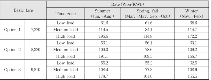
Since many electric motors are used to move water between the processes shown in Fig. 1, a significant amount of electricity is consumed. H purification plant must pay the electricity charge based on the Industry B rate provided by KEPCO (Korea Electricity and Power Cooperation), which is shown in Table 1. The Industry B rate is applied to customers in the fields of manufac- turing, mining, etc. The unit is Korean Won (Won) per KWh.
Currently, H uses option 2 for its electricity rate. As shown in Table 1, Industry B rates have three different time zones of low, medium, and high electricity load, whose rates differ from each other. For instance, for option 2, the rate during high load is more than three times of that during low load in summer time, two and a half times in winter, and two times in spring and fall. Table 2 shows the seasonal time zones of low, medium, and high electricity load determined by KEPCO.
We can also see that time zones differ from season to season.
The most significant cost of water production is the electricity cost. To reduce the electricity cost we need
Basic fare
Rate (Won/KWh)
Time zone Summer
(Jun.~Aug.) Spring, fall
(Mar.~May, Sep.~Oct.) Winter (Nov.~Feb.)
Option 1 7,220
Low load 61.6 61.6 68.6
Medium load 114.5 84.1 114.7
High load 196.6 114.8 172.2
Option 2 8,320
Low load 56.1 56.1 63.1
Medium load 109.0 78.6 109.2
High load 191.1 109.3 166.7
Option 3 9,810
Low load 55.2 55.2 62.5
Medium load 108.4 77.3 108.6
High load 178.7 101.0 155.5
Table 1. Industry B Electricity Rate (KEPCO, 2015)
Time zone Spring, summer, fall Winter
(Mar.~Oct.) (Nov.~Feb.)
Low load 23:00~09:00 23:00~09:00
Medium load
09:00~10:00 12:00~13:00 17:00~23:00
09:00~10:00 12:00~17:00 20:00~22:00
High load 10:00~12:00
13:00~17:00
10:00~12:00 17:00~20:00 22:00~23:00 Table 2. Seasonal Time Zone (KEPCO, 2015)
to maximize clean water production during low loads and store water within the reservoir capacity so that we can meet the water demand during high loads without producing water.
2.3 Current Method for Determining Water Intake Amount
2.3.1 Estimation of Hourly Flow Amount The hourly flow amount (HFA) is the amount of water sent from the clean water reservoir to the demand area during an hour. Therefore, estimating the HFA provides an estimation of the water amount required during an hour in the demand area, which is calculated using a simple method as follows. On the hour, the amount of water flow during one second is measured and mul- tiplied by 3600.
H purification plant produces a daily flow report, which includes an estimated HFA, the real HFA, and the amount of hourly water intake from Paldang (H
Arisu Purification Center, 2013.9~2014.4). The real HFA is the measured amount of flow during an hour from the clean water reservoir to the demand area. H also produces a daily water level report, which is the important element for determining the amount of hourly water intake from Paldang.
2.3.2 Determination of Hourly Water Intake Amount from Paldang
An operator determines the water intake amount based on the estimated HFA and the water level of the clean water reservoir. After determining the water intake amount, the operator can obtain the desired amount of water by controlling the motor-operated valves of M-102A and M-102B. By considering the electricity rate of Tables 1 and 2, they can take more water than the estimated HFA during low loads so that they can meet the demand during high loads with less water intake. The deviation from the estimated HFA depends on the experience and skill of the operator.
During this operation, the water level must be main- tained above 3.1 m for water pressure and below 4.6 m, which is the maximum height of the reservoir.
2.4 The Problems of the Current Method Determining the hourly water intake amount is based on the hourly estimation of HFA. Since HFA is esti- mated by measuring the amount of water that flows during one second times 3600, its accuracy cannot be guaranteed. The daily flow report from H shows the estimated and measured HFAs. Smaller differences between these two values suggest a more accurate esti- mation. To see the difference, a t-test was performed with the data from the daily flow report and there was a difference at a significance level of 0.05 (t=3.32, DOF=
862). Since the estimation of the HFA is not accurate, the hourly amount of water intake cannot accurately meet the water requirement of the demand area.
The arriving water in the deposit basin is not directly supplied to customers. It undergoes a six-hour pro- duction process as shown in Fig. 1 before being sup- plied to customer. This means that the water taken from the intake station cannot be used to meet instan- taneous demand, but the demand after with a delay of six hours. The current method, which estimates HFA on the hour and determines the amount of water intake based from that estimated value, is adequate from the viewpoint of meeting daily water requirement. However, it is not adequate from the viewpoint of minimizing electricity cost, which is the most significant cost of water production. For instance, let us suppose that we want to estimate the amount of water intake at 11:00 A.M.
during high load and the HFA for this time is estimated to be very large. We also suppose that the water demand will be very low after six hours, when the water taken at 11:00 A.M is supplied to the customer. In this case, from the viewpoint of minimizing electricity cost, it is not a good decision to determine the amount of water intake based on the HFA estimated for the same hour.
Of course, when operators determine the water intake amount based on the HFA estimate, they consider the electricity rates for different time zones and adjust the intake amount accordingly. However, since this adjust- ment is largely based on the experience and skill of the operator, there is no consistency among the operators, who work in three eight-hour shifts. In addition, while meeting time-varying demand and maintaining the
proper water level in the clean water reservoir, the methodology for minimizing electricity cost when dealing with different electricity rate time zones is a very com- plicated problem, and addressing it is beyond the operator’s experience and skill.
2.5 The Proposed Method
In this study, an LP model is proposed that can mini- mize the daily electricity cost while meeting time-varying demand. The objective function is the minimization of the daily electricity cost, and the hourly amount of water taken from the water intake station is the decision variable. All of the constraints and the detailed model will be discussed in next chapter. The hourly water demand required for input in the LP model is obtained from a demand forecast based on previous data. By doing so, we can determine the amount of water intake from Paldang based on the forecast value of the water demand for six hours later. The data used in this study are estimated HFA, measured HFA, and real intake water amount on December 20th, 2013 and April 20th, 2014, which are obtained from the daily flow report from H.
3. LP Model Development 3.1 Basic Input Data
3.1.1 Hourly Water Usage Estimate
The most important input data for the LP model is the hourly water usage estimate. For arriving at an accurate estimate, it is important to select a proper estimation method. In this study, the exponential smoo- thing technique with a constant of 0.2 is used [1,2].
The estimation results are shown in Chapter 4. The effect of the forecast accuracy on the LP solution will be discussed in Chapter 5 in more detail. To reduce the variation of the estimated hourly demand, the estimate is normalized using the monthly average water demand.
3.1.2 Electricity Cost
Time zone based electricity rates are shown in Tables 1 and 2. It takes six hours to produce clean water, which is the delay from the water intake station to the clean water reservoir. Thus, we should consider the time-varying electricity rate in six-hour spans. In this study, for simplicity, the average electricity rate for
Time ACi(April) ACi(December) Time ACi(April) ACi(December)
0 56.10 63.10 12 99.07 128.37
1 56.10 63.10 13 99.07 137.95
2 56.10 63.10 14 93.95 147.53
3 56.10 63.10 15 88.83 157.12
4 59.85 70.78 16 83.72 166.70
5 68.72 88.05 17 78.60 149.43
6 77.58 105.32 18 74.85 132.17
7 81.33 113.00 19 71.10 114.90
8 90.20 120.68 20 67.35 97.63
9 99.07 128.37 21 63.60 80.37
10 104.18 118.78 22 59.85 63.10
11 104.18 118.78 23 56.10 63.10
Table 3. ACi(Won/KWh)
Reservoir Dimension (m) Capacity (m3)
1 (65, 55, 4.6) 16,445
2 (65, 55, 4.6) 16,445
3 (65, 55, 4.6) 16,445
4 (65, 55, 4.6) 16,445
5 (55, 52.5, 4.6) 13,282.5
6 (55, 52.5, 4.6) 13,282.5
7 (65, 55, 4.6) 16,445
8 (65, 55, 4.6) 16,445
9 (70, 50, 4.6) 16,100
10 (70, 50, 4.6) 16,100
11 (70, 65, 4.6) 20,930
Total capacity 178,365
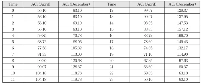
Table 4. Dimension of Reservoirs (H Arisu Purification Center, 2015) the next six hours is used. That is, the electricity rate
ACiapplied to the water taken from the intake station at time i can be calculated as follows:
(1) ACifor April and December is shown in Table 3. The unit is Won (Korean Won)/KWh.
3.1.3 Electricity Required to Produce 1 m3of Clean Water
The electricity required K to produce 1 m3of clean water can be obtained by dividing the total electricity used during a month by the total amount of water pro- duced during the month. For instance, the total electricity used in April, 2014 was 501,066 KWh and the
total amount of water produced was 6,512,300 m3, so K becomes 0.07694 KWh.
3.1.4 Size of the Clean Water Reservoir H has eleven reservoirs that store clean water before it is supplied to the customer. Their dimensions are shown in Table 4. To send water to the customer, the water level in the clean water reservoir must be maintained above 3.1 m. The water level should also be kept below 4.6 m, which is the maximum height of the reservoir.
3.2 Assumptions
1) It takes six hours to produce water, so it is assumed the water taken from the water intake station can
be used to meet the demand after six hours.
2) As mentioned previously, the electricity rate to produce water taken at time i (i=0,1,2,…,23) is determined as the average of electricity rates for next six hours.
3) We assume that the produced water is evenly distributed among the eleven reservoirs. Through this assumption, we do not treat each reservoir separately, but as one big reservoir with a bottom area of 38,775 m2(178,365 m3/4.6 m) and a height of 4.6 m.
4) The water level in the reservoir must be kept above 3.1 m and below 4.6 m. It is almost impos- sible to check these requirements at all times in the model. Instead, we check these requirements only on the hour.
5) In this study, we do not consider other production costs such as inventory cost, labor cost, proces- sing cost, etc.
3.3 LP Model
Pi is the decision variable, which represents the amount of water taken from the Paldang intake station at time i (i=0,1,2,…,23). Our objective function is the minimization of the daily electricity cost. That is,
. (2)
There are several constraints for our linear program- ming model. That is,
a. Remaining water in the reservoir
We let Wi represent the remaining water in the reservoir at the beginning of hour i, and we let Direp- resent the water demand forecast during time (i, i +1).
Then Wi+1 can be calculated as the summation of Wi
and Pi-6(water taken six hours before and arriving at the reservoir at the beginning of hour i) and then subtracting Di. That is,
(3) In this equation, if (i-6) has negative value, we add 24. This accounts for a 24-hour cycle. For instance, W2
=W1+P19-D1, where P19represents the amount of water intake determined from the LP model a day before.
b. Water level constraint
On the hour, the height of the clean water reservoir is Wi/38,775 (m2). This height should be above 3.1 m to secure water pressure and below the maximum height
of the reservoir (4.6 m). That is,
(4a) (4b) c. Limitation of water intake amount
The hourly amount of water taken from the water intake station cannot exceed 15,000 m3. That is,
(5)
4. Real-field Example 4.1 Data
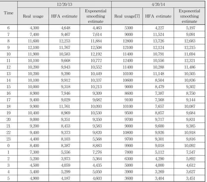
Table 5 shows the hourly real water usage, HFA estimate, and exponential smoothing estimate on December 20th, 2013 and April 20th, 2014. The hourly real usage and HFA estimate are obtained from the daily flow report from H, and the exponential smoo- thing estimate is calculated based on past data (Agresti, 1996 and Box et al., 1998). Our goal is to determine Pi
from time 0:00 to time 23:00 on the 20th, which is based on data from 06:00 on the 20thto 05:00 on the 21st. Table 6 shows the data for that period. Real usage data came from H Arisu Purification Center (2013.9~2014.4).
4.2 Results
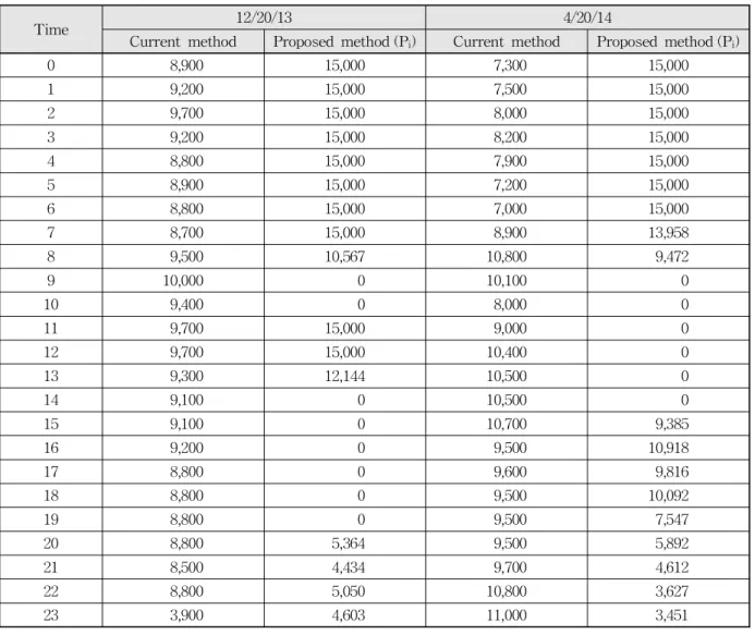
Using the LP model developed in Chapter 3 and the exponential smoothing estimate from Section 4.1, the optimal hourly water intake amounts (Pi) from Paldang are derived, and results are summarized in Table 6. The water intake amounts of the current method are obtained from the daily flow report from H, and Pi is obtained from the Excel Solver.
We can see that the Pi’s in Table 7 are determined considering the ACiin Table 4. That is, when the aver- age electricity rate at time i (ACi) is low, more water is taken and vice versa. A maximum of 15,000 m3is taken during periods with low ACi, and none is taken during periods with high ACi.
The daily electricity costs of the current and proposed methods are compared in Table 7, which shows the daily electricity costs of the proposed method are 460,284 KW (Korean Won) less on December 20th and 350,936 KW less on April 20ththan those of the current one. Therefore, the proposed method using LP brings cost reductions of 25.38% and 25.45%, respectively.
Time
12/20/13 4/20/14
Real usage HFA estimate Exponential smoothing
estimate Real usage[7] HFA estimate Exponential smoothing
estimate
6 4,300 4,648 4,463 5300 4,227 5,197
7 7,400 9,467 7,614 9000 11,524 9,091
8 11,600 12,253 11,884 12800 13,726 12,683
9 12,100 11,767 12,508 12100 12,124 12,215
10 11,900 10,583 12,192 11400 10,791 11,694
11 10,100 9,668 10,772 12400 10,556 12,321
12 10,200 9,943 10,552 11400 10,288 11,486
13 10,200 9,390 10,449 10100 11,148 10,505
14 10,100 9,912 10,337 10600 8,504 10,836
15 10,000 9,318 10,213 9000 8,479 9,302
16 8,900 7,946 9,309 8600 7,387 8,750
17 9,400 9,029 9,682 9100 7,568 9,144
18 9,900 11,761 10,093 10100 7,657 10,087
19 10,400 8,969 10,530 9500 8,857 9,684
20 9,000 9,351 9,350 9700 9,717 9,831
21 9,200 8,453 9,583 9000 9,600 9,385
22 9,400 9,373 9,820 10800 9,926 10,918
23 4,400 8,103 5,568 9700 9,301 9,816
0 8,400 8,387 8,883 9900 9,018 10,092
1 7,300 5,556 7,276 7800 5,112 7,547
2 5,200 3,973 5,364 6300 4,290 5,892
3 4,500 4,059 4,435 5000 4,000 4,612
4 5,400 5,299 5,050 3900 3,269 3,627
5 4,900 4,187 4,603 3600 3,404 3,451
Table 5. Real Water Usage and Estimates (m3)
Under the current method, operators should monitor water levels continuously. They determine the hourly water intake amount from Paldang based on the HFA estimate, experience, and skill. This requires that operators should attend the site at all times. Under the proposed method using LP, however, operators need not always attend the site. Thus, labor cost reduction is also expected, but we will not explicitly consider this in this study as mentioned in the assumptions in Section 3.2.
The amount of water intake using the LP model is based on the water usage estimate of exponential smoo- thing. If the estimate is different from the real water usage, the water level can be below 3.1 m or above 4.6 m. Using the real water usage from the daily flow
report in Table 5 the hourly water levels under the two methods are calculated and shown in Table 8.
Under the current method, the water level is main- tained between 3.1 m and 4.6 m since the operator determines the water intake amount by monitoring the water level continuously. Unfortunately, under the pro- posed method, we can see water levels are higher than 4.6 m at 13:00, 14:00, and 18:00 on December 20th, 2013 and at 13:00 and 14:00 on April 20th, 2014. When ACiis low, the LP model tries to take as much water as possible, which leads to high water level around 4.6 m after 6 hours. However, when ACiis high, the LP model tries to take as little water as possible, which leads to a low water level around 3.1 m after 6 hours. Therefore, if the exponential smoothing estimate is different from
12/20/13 4/20/14
Current method Proposed method Current method Proposed method
1,813,412 1,353,128 1,378,857 1,027,921
Table 7. Comparison of Electricity Cost (Won)
Time 12/20/13 4/20/14
Current method Proposed method (Pi) Current method Proposed method (Pi)
0 8,900 15,000 7,300 15,000
1 9,200 15,000 7,500 15,000
2 9,700 15,000 8,000 15,000
3 9,200 15,000 8,200 15,000
4 8,800 15,000 7,900 15,000
5 8,900 15,000 7,200 15,000
6 8,800 15,000 7,000 15,000
7 8,700 15,000 8,900 13,958
8 9,500 10,567 10,800 9,472
9 10,000 0 10,100 0
10 9,400 0 8,000 0
11 9,700 15,000 9,000 0
12 9,700 15,000 10,400 0
13 9,300 12,144 10,500 0
14 9,100 0 10,500 0
15 9,100 0 10,700 9,385
16 9,200 0 9,500 10,918
17 8,800 0 9,600 9,816
18 8,800 0 9,500 10,092
19 8,800 0 9,500 7,547
20 8,800 5,364 9,500 5,892
21 8,500 4,434 9,700 4,612
22 8,800 5,050 10,800 3,627
23 3,900 4,603 11,000 3,451
Table 6. Hourly Amount of Water Intake from Paldang (m3)
the real water usage, the water level can exceed 4.6 m or drop below 3.1 m. The methods to handle this pro- blem will be discussed in Chapter 5.
5. Problems in the LP Model due to Inaccurate Estimates
To determine the optimal amount of water intake, the LP model uses an estimate of the hourly water usage in the demand area. If this estimate is not accurate, we can violate the water level constraints as shown above.
There might be two methods to handle this problem:
accurate estimates and safety margin.
5.1 Accurate Estimates
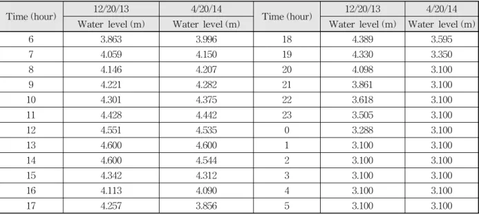
If an estimate is accurate, the water level is always maintained between 3.1 m and 4.6 m owing to the con- straints in the LP model. Let us suppose the real water usage in Table 5 is known beforehand and is used as input estimate data, which is impossible in reality. The water level and daily electricity cost are shown in Tables 9 and 10.
Time (hour) 12/20/13 4/20/14
Current method Proposed method Current method Proposed method
6 3.705 3.863 3.797 3.996
7 3.752 4.059 3.758 4.150
8 3.703 4.146 3.635 4.207
9 3.628 4.221 3.534 4.282
10 3.548 4.301 3.444 4.375
11 3.517 4.428 3.310 4.442
12 3.481 4.551 3.196 4.535
13 3.442 4.675 3.165 4.634
14 3.427 4.687 3.170 4.605
15 3.427 4.429 3.199 4.373
16 3.440 4.440 3.183 4.151
17 3.448 4.584 3.181 3.916
18 3.442 4.716 3.188 3.656
19 3.414 4.521 3.214 3.411
20 3.417 4.289 3.235 3.161
21 3.414 4.051 3.279 3.171
22 3.409 3.809 3.245 3.174
23 3.522 3.695 3.243 3.177
0 3.533 3.479 3.232 3.182
1 3.571 3.291 3.276 3.175
2 3.664 3.295 3.359 3.165
3 3.767 3.293 3.480 3.155
4 3.855 3.284 3.658 3.148
5 3.829 3.276 3.849 3.144
Table 8. Hourly Water Level (m) in the Reservoir
Time (hour) 12/20/13 4/20/14
Time (hour) 12/20/13 4/20/14
Water level (m) Water level (m) Water level (m) Water level (m)
6 3.863 3.996 18 4.389 3.595
7 4.059 4.150 19 4.330 3.350
8 4.146 4.207 20 4.098 3.100
9 4.221 4.282 21 3.861 3.100
10 4.301 4.375 22 3.618 3.100
11 4.428 4.442 23 3.505 3.100
12 4.551 4.535 0 3.288 3.100
13 4.600 4.600 1 3.100 3.100
14 4.600 4.544 2 3.100 3.100
15 4.342 4.312 3 3.100 3.100
16 4.113 4.090 4 3.100 3.100
17 4.257 3.856 5 3.100 3.100
Table 9. Water Level under Accurate Estimate
12/20/13 4/20/14
Current method Accurate estimate Current method Accurate estimate
1,813,412 1,286,518 1,378,857 1,025,870
Table 10. Comparison of Daily Electricity Cost (Won)
Date Electricity
cost(I)(won) Electricity
cost(II)(won) Electricity
cost(III)(won) Lowest water
level(II)(m) Highest water level(II)(m)
December 20th, 2013 1,813,412 1,353,128 1,286,631 3.276 4.716
April 15th, 2014 1,313,121 1,008,598 960,295 3.030 4.554
Table 11. Electricity Cost and Water Level
From Table 9, we can see that water levels are al- ways maintained above 3.1 m and below 4.6 m if the LP model uses the real water usage of Table 5 as its esti- mates. We can also see a cost reduction of 29.06%
(526,894 KW) on December 20th, 2013 and 25.6%
(352,987 KW) on April 20th, 2014.
However, it is almost impossible to estimate the real amount of water usage accurately. It is important to select the best estimation method by comparing different ones.
However, it is worrying that an in-depth study and discussion about forecast techniques might distract from the overall flow of this study. In addition, no matter how good a forecast technique is, there is always error, which brings the potential of violating the water level constraint. Therefore, keeping the exponential smoothing method, we propose a ‘safety margin’ method which can accommodate the estimate inaccuracy.
5.2 Safety Margin 5.2.1 Safety Margin
To keep the water level between 3.1 m and 4.6 m under inaccurate estimates for the hourly water usage, safety margins k1and k2are introduced. The minimum height is changed to 3.1*(1+k1), and the maximum height is changed to 4.6*(1-k2). Data from December 15thand 20th, 2013 and April 15th and 20th, 2014 are used to see the effects of k1 and k2.
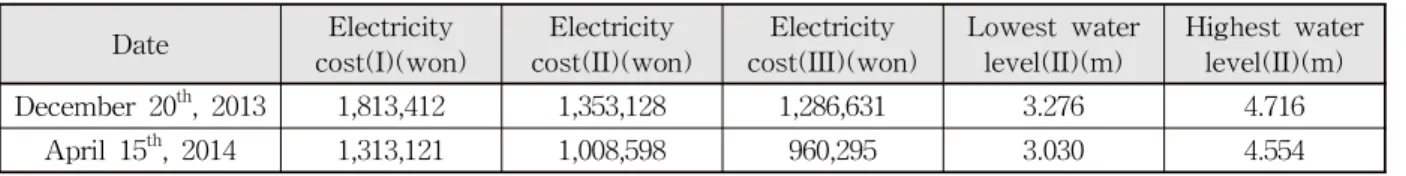
Using the data from December 20th, 2013 and April 15th, 2014, k1and k2are derived, which can satisfy water level constraints. Table 11 shows the daily electricity cost and the water level of the reservoir when k1 and k2are not used.
In Table 11, method I is the current method, and method II uses the proposed LP model and an expon-
ential smoothing estimate. Method III uses the proposed LP model and real data as an estimate, which is most accurate but impossible in reality. Method III gives upper bounds for the electricity cost reductions that method II can attain.
For both days, the proposed method brings signi- ficant cost reductions (25.38% on December 20th and 23.19% on April 15th) compared with the current method, and its daily electricity costs are just slightly higher than that of method III (5.17% on December 20th and 5.03% on April 15th). However, the proposed method cannot be used because the maximum water level (4.6 m) is violated on December 20thand the minimum water level (3.1 m) is violated on April 15th.
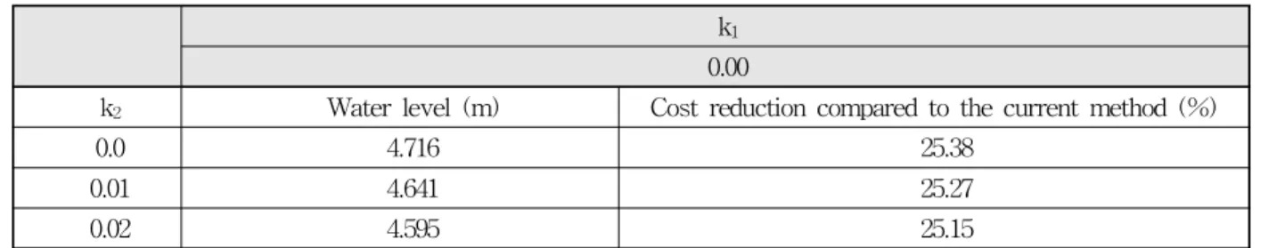
For December 20th, we need to introduce the safety margin k2. Thus, in the LP model, the water level should be lower than 4.6*(1-k2). Table 12 shows thatthe maxi- mum water level is satisfied with k2=0.02, and we can still attain 25.15% cost reduction compared to the current method.
For April 15th, the safety margin k1is needed. Thus, in the LP model, the water level should be higher than 3.1*(1+k1). Table 13 shows that the minimum water level is satisfied with k1=0.03, and we can still attain 14.74% cost reduction compared to the current method.
Based on the 15th and 20th of April 2014, the upper bounds of k1and k2are obtained, which can secure cost reduction compared to the current method without violating water level constraints. For April 15th, the safety margin k1is needed and its upper bound is determined as 0.1975. That means we can still secure electricity cost reduction and keep the water level above 3.1 m even though 3.71 m (3.1*(1+0.1975)) is used for the minimum water level instead of 3.1 m. Using the LP model with k1=0.1975, the lowest water level becomes 3.642 m. Even
k1=0.05 (4.37 m) k1=0.1 (4.14 m) k1=0.15 (3.91 m) k2=0.05 (3.26 m) 1,547,231 (18.31%) 1,602,969 (15.37%) 1,661,523 (12.27%) k2=0.1 (3.41 m) 1,553,243 (17.99%) 1,746,593 (7.78%) 1,835,040 (3.11%) k2=0.15 (3.57 m) 1,700,193 (10.23%) 1,819,314 (3.94%) 1,836,046 (3.06%) Table 14. Electricity Cost Reduction according to Combination k1 and k2(December 15th, 2013)
k1
0.00
k2 Water level (m) Cost reduction compared to the current method (%)
0.0 4.716 25.38
0.01 4.641 25.27
0.02 4.595 25.15
Table 12. Water Level and Cost Reduction according to k2(December 20th, 2013)
k2
0.00
k1 Water level (m) Cost reduction compared to the current method (%)
0.0 3.030 23.19
0.01 3.065 22.54
0.02 3.091 21.87
0.03 3.123 14.74
Table 13. Water Level and Cost Reduction with Respect to k1(April 15th, 2014)
if we have forecast error in the exponential smoothing estimate for the water usage, the water level is main- tained above 3.1 m. For April 20th, the safety margin k2
is needed and its upper bound is determined as 0.190.
That means we can still secure electricity cost reduction and keep the water level below 4.6 m even though 3.73 m=(4.6*(1-0.19)) is used for the maximum water level instead of 4.6 m. Using the LP model with k2=0.190, the highest water level becomes 3.745 m. Even if we have forecast error in the exponential smoothing estimate for the water usage, the water level is maintained below 4.6 m.
When the LP model is used to determine the hourly water intake amount, we do not know which water level constraint (maximum, minimum, or both) is violated.
Therefore, we need to simultaneously use both k1and k2. Using the data from December 15th, 2013 and April 15th, 2014 we show the daily electricity cost reductions compared to the current method according to various combinations of k1 and k2, and results are shown in Tables 14 and 15. All of the combinations satisfy the water level constraints. We can see daily cost reduc- tions in the range of of 3.06-18.31% on December 15th,
2013 and 2.68~8.37% on April 15th, 2014. For instance, if both k1 and k2are set as 0.1 (i.e., 4.14 m instead of 4.60 m maximum and 3.41 m instead of 3.10 m minimum), the cost reduction is 7.78% on December 15th, 2013 and 6.03% on April 15th, 2014.
As seen in the several examples above, the upper bounds of safety margins k1and k2are relatively large, which can secure cost reduction compared to the current method without violating water level constraints. This means that safety margins k1and k2can practically and safely solve the water level violation problem that is due to inaccurate estimates for the water usage in the demand area.
5.2.2 Safety Margin and Inaccurate Estimate In section 5.2.1, safety margins were proposed to solve the water level violation problem under the exponen- tial smoothing estimate. Since the estimate accuracy is never guaranteed, we need to investigate the effect of inaccurate estimates on k1and k2. To do this, we take the daily average of the water usage in April 2014. Assuming hourly water usage is uniform, we just divide the daily
Current method LP using the exponential smoothing estimate LP using the inaccurate estimate Cost (won) Cost (won) Maximum water level (m) K2 Cost (won) Maximum water level (m) K2
1,378,857 1,027,921 4.634 0 1,117,901 4.696 0
1,029,259 4.594 0.01 1,121,974 4.576 0.06
Table 17. Effect of Inaccurate Estimate on Safety Margin (April 20th)
k1=0.05 (4.37 m) k1=0.1 (4.14 m) k1=0.15 (3.91 m) k2=0.05 (3.26 m) 1,203,297 (8.37%) 1,203,738 (8.34%) 1,210,881 (7.79%) k2=0.1 (3.41 m) 1,225,226 (6.70%) 1,234,085 (6.03%) 1,241,701 (5.45%) k2=0.15 (3.57 m) 1,249,958 (4.82%) 1,273,350 (3.04%) 1,278,032 (2.68%) Table 15. Electricity Cost Reduction according to Combination k1 and k2(April 15th, 2014)
Current
method LP using the exponential
smoothing estimate LP using the inaccurate estimate (won)Cost Cost
(won) Minimum
water level (m) k1 Cost
(won) Minimum
water level (m) Maximum
water level (m) k1 k2
1,313,121 1,008,598 3.03 0 1,099,333 3.042 4.668 0 0
1,119,691 3.123 0.03 1,120,877 3.104 4.560 0.05 0.02
Table 16. Effect of Inaccurate Estimate on Safety Margin (April 15th)
average by 24 for the estimate of the hourly water usage.
This is very inaccurate and is called the ‘inaccurate estimate’ in this study. The daily average is 215,082 m3 in April and the hourly water usage is estimated as 8,961.75 m3(215,082/24).
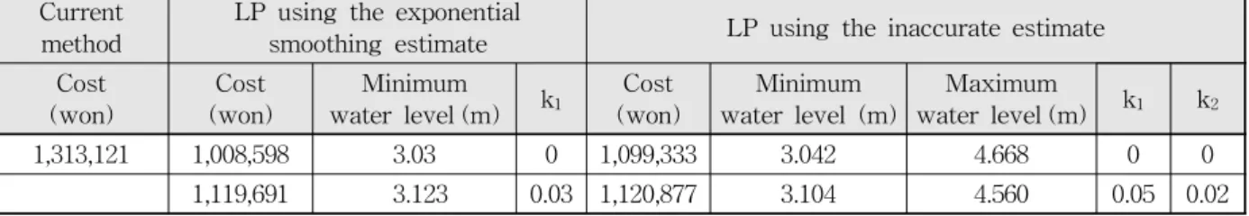
Based on the data from April 15th and 20th2014, the daily electricity cost and safety margin k1and k2 are compared under three different methods and shown in Tables 16 and 17. For April 15th, the LP model using the exponential smoothing estimate satisfies the minimum water level when k1=0.03, and the daily electricity cost is 1,119,691 KW. Under the inaccurate estimate, the minimum water level is satisfied when k1=0.05 and k2= 0.02, and the daily electricity cost is 1,120,877 KW. The inaccurate estimate slightly increases the cost compared with the exponential smoothing estimate but can still secure a cost reduction of 14.6% compared with the current method. For April 20th, the LP model using the exponential smoothing estimate satisfies the minimum water level when k2=0.01, and the daily electricity cost is 1,029,259 KW. Under the inaccurate estimate the mini- mum water level is satisfied with a daily electricity cost of 1,121,974 KW when k2=0.06. The inaccurate estimate slightly increases the cost compared with the exponen- tial smoothing estimate but can still secure a cost
reduction of 15.1% compared with the current method.
As seen in the previous two examples, satisfying the water level constraints under inaccurate estimate requires larger values for the safety margins k1and k2, which leads to increases in electricity cost. However, inaccurate estimates can still secure significant cost reduction compared with the current method. This sug- gests that the safety margin method still works effec- tively under inaccurate estimates for hourly water usage.
6. Conclusion
A LP model was proposed, which can determine the optimal hourly water intake amount for minimizing the daily electricity cost. The input data of the LP model is obtained from the daily flow report from H. To estimate hourly water usage in the demand area, the exponential smoothing method with a constant of 0.2 is used. We can secure a significant cost reduction (25.38% on December 20th 2013 and 25.45% on April 20th 2014) through the LP method using the exponential smoo- thing estimate. Operators need not attend to the site at all times under the proposed LP method, and we can additionally expect reductions in labor costs.
It was shown that an inaccurate estimate for the
hourly water usage in the demand area causes the water level constraint to be violated, which is the weak point of the proposed LP method. However, several examples with real-field data show that we can practically and safely solve this problem with safety margins. It was also shown that safety margin method still works effec- tively whether the estimate is accurate or not.
All of the discussions about safety margin are based on the data from December 15thand 20th, 2013 and April 15th and 20th, 2014, so our assertion might not hold generally. Through several examples, however, it is shown that the upper bounds of the safety margins are relatively large, which can secure cost reduction com- pared with the current method without violating water level constraints. This means that safety margins can be used practically and safely, even in the generic case.
If safety margins are combined with an accurate esti- mation method, the effectiveness of the LP method will be further increased.
Acknowledgments
This study was supported by the research program funded by the Seoul National University of Science and Technology.
References
(http://arisu.seoul.go.kr/arisu_center/center1/sub1_3.jsp).
(http:/cyber.kepco.co.kr/ckepco/front/jsp/CY/E/E/CYE EHP00103.jsp).
Agresti, A. (1996). “An Introduction to categorical data an- alysis. (1st ed.).” Florida : John Wiley & Sons, (Chapter 4).
Box, G.E.P., and Draper, N.R. (1998). “Evolutionary opera- tion: a statistical method for process improvement.
(2nd ed.).” WILEY, (Chapter 2).
Ferreira, A.R., and Teegavarapu, R.S.V. (2012). “Optimal and adaptive operation of a hydropower system with unit commitment and water quality constraint.”Water Resources Management, Vol. 26, No. 3, pp. 707-732.
H Arisu Purification Center (2015). “Major operational plan.”
H Arisu Purification Center 1) (2013.9~2014.4). “Daily electrical power report.”
H Arisu Purification Center 2) (2013.9~2014.4). “Daily flow report.”
H Arisu Purification Center 3) (2013.9~2014.4). “Daily water level report.”
Han, Y., Huang, Y., Jia, S., and Liu, J. (2013). “An interval parameter fuzzy linear programming with stochastic vertices model for water resource management under uncertainty.”Mathematical Problems in Engineering, Vol. 2013, Article ID 942343, 12 pages.
Heydari, M., Othman, F., and Quaderi, K. (2015). “Intro- duction to linear programming as a popular tool in optimal reservoir operation, a review.” Advances in Engineering Biology, Vol. 9, No. 3, pp. 906-917.
Heydari, M., Othman, F., Quaderi, K., nori, M., and Shahirparsa, A. (2015). “Developing optimal reservoir operation for multiple and multipurpose reservoirs using mathematical programming.” Mathematical Problems in Engineering, Vol. 2015, Article ID 435752, 11 pages.
Jung, J.K., and Lee, K.W.(2014). “Study on the optimal design of microgrid system using linear program- ming.”Journal of the Korea Management Engineers Society, Vol. 19, No. 4, pp. 59-74.
KEPCO (2015). “Electricity Rate Table.”
Mena, J.A. (2012). “The optimal organization structure design problem in make-to-order enterprises.”Inter- national Journal of Industrial Engineering, Vol. 19, No. 4, pp. 181-192.
Morais, H., Kadar, P., Faria, P., Vale, A., and Khodr. H.
(2010). “Optimal scheduling of a renewable microgrid in an isolated load area using mixed-integer linear programming.”Renewable Energy, Vol. 35, No. 1, pp.
151-156.
Tseng, T.L., Rosales, C.L., and Kwon, Y.J. (2014). “Opti- mization of wind turbine placement layout on non-flat terrains.” International Journal of Industrial Engi- neering, Vol. 21, No. 6, pp. 384-395.
Zhao, T., and Zhao, J. (2014). “Optimization operation of water supply reservoir: the role of constraints.”
Mathematical Problems in Engineering, Vol. 2014, Article ID 853186, 15pages.
paper number : 15-074 Received : 11 September 2015
Revised : 16 October 2015 / 23 October 2015 Accepted : 23 October 2015