ABSTRACT
In this paper, we propose a novel dynamic subchannel grouping (DSG) algorithm to maximize the system capacity considering intended proper outage probability for the downlink of enterprise small-cell networks (ESNs). In the proposed DSG scheme, a local gateway (LGW) which is installed in a building dynamically divides the frequency bandwidth into different numbers of subchannel groups (SGs) based on the numbers of small-cell access points (SAPs) and small-cell user equipments (SUEs) per floor. Then, the LGW assigns the SGs to SAPs and the SAPs allocate them to their serving SUEs. Through simulation results, we show that the proposed DSG scheme is appropriate for the ESNs compared to the conventional small-cell networks in which all SAPs use the number of fixed SGs in terms of the system capacity and outage probability.
☞ keyword : Small-cell networks, Enterprise, Local gateway, Dynamic, Subchannel grouping
1. Introduction
Recent technological advances in mobile devices, e.g., smart phones, tablet PCs, and so on, have red to increase wireless data traffic explosively [1][2][3]. Further, more than half of the traffic occur indoor environment during daytime [4] and small-cell networks have become an attractive solution to extend the coverage of conventional cellular networks (CCNs) with providing high speed data service [5][6][7][8][9]. Thus, the world’s major mobile network operators (MNOs) currently show a great deal of attention to adopt small-cells for the enterprise environments, i.e., enterprise small-cell networks (ESNs), because a lot of people work in their companies during daytime and it means that ESNs are more useful than residential small-cell networks (RSNs) in which one or two small-cell access
1 Dept. of Computer Science and Statistics, Chosun University, Gwangju 61452, Korea.
* Corresponding author ([email protected])
[Received 5 August 2017, Reviewed 14 August 2017(11 October 2017), Accepted 1 November 2017]
☆ This work was supported by the National Research Foundation of Korea (NRF) Grant funded by the Korean Government (MSIP) (No. 2015R1C1A1A01055869).
points (SAPs) are installed in each detached house [10][11][12][13][14]. However, in ESNs, a lot of SAPs are densely installed in a building and they serve different numbers of small-cell user equipments (SUEs) with strong interference from neighbor SAPs. Most work have been studied about small-cell networks are for RSNs and a couple of work have been studied for ESNs [15][16]. In [15], authors proposed a load sharing scheme using a handover margin and transmit power managements based on fuzzy logic controller. On the other hand, in [16], authors proposed an adaptive sub-band allocation scheme based on the interference graph. However, both schemes in [15] and [16]
use distributed methods and thus every SAP needs to check the traffic load and interference of adjacent SAPs to use those schemes.
In this paper, we propose a novel dynamic subchannel
grouping (DSG) algorithm to maximize the system capacity
considering intended proper outage probability for the
downlink (DL) of ESNs. In the proposed DSG scheme, a
local gateway (LGW) which is installed in a building
dynamically divides the frequency bandwidth into different
numbers of subchannel groups (SGs) based on the numbers
of SAPs and SUEs per floor. Then, the LGW assigns the
SGs to SAPs and the SAPs allocate them to their serving
(Figure 1) System architectures of RSNs and ESNs
SUEs. Through simulation results, we show that the proposed DSG scheme is appropriate for the ESNs compared to the conventional small-cell networks in which all SAPs use the number of fixed SGs in terms of the system capacity and outage probability.
The remainder of this paper is organized as follows.
Section 2 introduces various system models and Section 3 explains the proposed DSG scheme using the LGW. Then, Section 4 evaluates the system performance and section 5 concludes this paper with future research direction.
2. System Model
2.1 System architectures for ESNs Fig. 1 shows system architectures of RSNs and ESNs [10][11]. As shown in Fig. 1-(a), the RSN consists of SAPs, SUEs, and a small-cell gateway (SGW) and they are added to the CCN that has two components, i.e., macro base stations (MBSs) and macro user equipments (MUEs).
Further, all SAPs are connected to the MNO’s core network through the Internet and SGW and then the SGW manages all SAPs for the initial configuration, channel allocation, handover, and so on. However, each SGW manages up to 1000 SAPs and thus the architecture is appropriate for RSNs since each detached house has one or more SAPs in RSNs.
On the other hand, as shown in Fig. 1-(b), in ESNs, a lot of SAPs and SUEs are deployed in a building and a LGW is added to the architecture of ESNs to manage the SAPs and
SUEs instead of the SGW with low transmission delay [17].
That is, the LGW dynamically assigns SGs to SAPs based on the numbers of SAPs and SUEs.
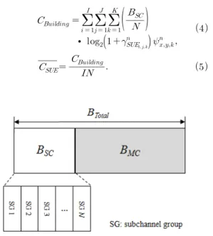
Small-cell networks consider two kinds of bandwidth allocation schemes, i.e., shared reuse and split reuse [18]. In the shared reuse scheme, the total frequency bandwidth, B
Total, is used by both MUEs and SUEs at the same time while in the split reuse scheme, B
Totalis divided into two groups for the macrocell and small-cell networks, B
MC, and B
SC, and thus there is no interference between MBSs and SAPs. In this paper, we use the split reuse scheme because the shared reuse scheme has different performance results according to the distance between the MBS and buildings with ESNs. Further, for ESNs, we consider a square topology of each floor and the width of the building is W
Buildingwhile the number of total floors in a building is I and the height of each floor is H
Floor. The gap between floors and the height of SAPs are H
Gapand H
SAP, respectively. In each floor, J SAPs are installed in grid patterns and K SUEs are uniformly distributed. The SGW and LGW divide B
SCinto N SGs and send this information to SAPs in RSNs and ESNs, respectively. Then, the SAP randomly allocates different SGs to their serving SUEs (one SG to one SUE).
2.2 Channel and SINR models
We consider a path loss model between the SAP and
SUE, PL, as shown in (1).
(Figure 2) N SGs in B
SCfor the split reuse.
Let
be the SINR of the k-th SUE (1≤k≤K) serviced by the j-th SAP (1≤j≤J) on the i-th floor (1≤i≤I) for the n-th SG (1≤n≤N). Then,
, can be expressed as (2).
≠
∙
where,
is the strength of the received signal of the k-th SUE served by the j-th SAP on the i-th floor for the n-th SG while
is the strength of interfering signals to the k-th SUE from the y-th SAP (1≤y≤J) on the x-th floor (1≤x≤I) for the n-th SG. Further, N
0is the white noise power and
is a binary indicator,
=1 if the y-th SAP on the x-th floor uses the n-th SG for the k-th SUE and 0 otherwise.
2.3 System capacity and outage probability
After obtaining
, we can analyze the capacity of the k-th SUE served by the j-th SAP on the i-th floor,
, using the Shannon theorem as expressed in (3).
(3)
Then, the capacity of all SAPs in the building, , and the average capacity of the SUE, , are calculated by (4) and (5), respectively.
Further, we evaluate the outage probability for SUEs,
, as expressed in (6).
≈
∙
where, and are the numbers of SUEs that have SINR values less than the SINR threshold, , and SUEs that receive no SG from their serving SAPs because the number of SUEs served by their SAPs is greater than the number of SGs, respectively.
3. Proposed DSG Scheme using the LGW
Fig. 2 shows the bandwidth allocation for the split reuse in small-cell networks. The SAPs use B
SCin B
Totalfor SUEs.
In RSNs, the SGW divides B
SCinto N SGs that are fixed,
e.g., N is 5, 10, or 20 SGs. Thus, the number of SUEs that
receive no SG from their serving SAPs can be increased as
N decreases. On the other hand, in the proposed DSG
scheme, the LGW knows the numbers of SAPs and SUEs in
the building by exchanging control messages between the
N (3x3, J=9) N (5x5, J=25)
1 ( ) 10 5 5
2 20 10 10
3 30 15 10
4 40 20 15
5 ( ) 50 25 15
(Table 1) N according to in the proposed DSG scheme
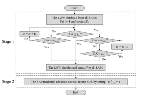
(Figure 3) A flow chart for the proposed DSG scheme using the LGW.
LGW and SAPs, periodically. Then, the LGW dynamically divides B
SCinto different numbers of SGs, i.e., N is different based on the numbers of SAPs and SUEs per floor in the building of EFNs. Further, the amount of the frequency bandwidth per SG is depend on N, i.e., B
SC/ N. That is, the amount of the frequency bandwidth per SG decreases as N increases and vice versa.
Fig. 3 shows a flow chart for the proposed DSG scheme using the LGW. The proposed DSG scheme consists of two stages. In stage 1, the LGW obtains J and counts K using control messages from all SAPs. Then, the LGW increases and decreases N when K becomes over and lower than the previously defined number of SUEs, , respectively. Here,
is the level between 1 and 5 for . For example, the LGW increases based on J and K and then sends a control message with N to all SAPs to update when K exceeds the specific numbers of SUEs in that are different according to J, i.e. 3×3 (9 SAPs) or 5×5 (25 SAPs) grid pattern. On the other hand, in stage 2, SAPs assign N SGs to their serving SUEs but the SAP randomly allocates one SG with
⌊B
SC/N⌋ to one SUE. In other words, the serving SAP sets
=1 when the y-th SAP on the x-th floor allocates the n-th SG for the k-th SUE. Table 1 shows N according to in the proposed DSG scheme.
4. Performance Evaluation
We investigate the DL performance of the proposed DSG scheme in terms of the system capacity, outage probability, and resource utilization for ESNs using a Monte Carlo simulation. We performed 200 independent simulations to evaluate the system performance according to the different numbers of SUEs, SAPs, and SGs in the analysis. We assume that the building with EFNs is open space such as department stores and business buildings and thus a log-normal shadow fading is considered with zero mean and standard deviation of 4dB for the link between the SAP and SUEs [17]. The values of noise figure for SUE is 8dB and
=-6dB. Table 1 gives N according to in the proposed
DSG scheme and each level is already defined considering
intended proper outage probability less than the boundary of
H
Floor3m
H
Gap0.5m
H
SAP3m
SINR threshold ( ) -6dB Boundary of P
out0.05
N
0-174dBm/Hz
10 20 30 40 50
0.2 0.3 0.4 0.5 0.6 0.7 0.8 0.9 1
Total EFN capacity (Gbps)
Number of SUEs (K) RSN:5x5(5 SGs)
RSN:3x3(5 SGs) RSN:5x5(10 SGs) RSN:3x3(10 SGs) RSN:5x5(20 SGs) RSN:3x3(20 SGs) Prop.:5x5 Prop.:3x3
(Figure 6) Total capacity of SUEs in a building
Number of SUEs (K)
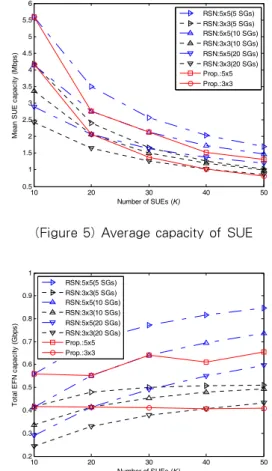
(Figure 5) Average capacity of SUE
0 10 20 30 40
50
0 10 20 30 40 50
0 2 4 6 8 10
X-width(m) Y-width(m)
Floor number
SAPs SUEs
(Figure 4) An example of deployment of 9 SAPs with the 3x3 grid pattern and 10 SUEs per floor in a building
. For example, the values of N are respectively 15 and 10 for the 3×3 and 5×5 grid pattern models in the proposed DSG scheme when =3, i.e., =30. Table 2 gives the key system parameters and Fig. 4 shows an example of deployment of 9 SAPs with the 3×3 grid pattern and 10 SUEs per floor in a building.
Fig. 5 describes the results of as the number of SUEs increases with different N. In both schemes, the capacity results decrease as K increases and the 5×5 grid pattern model has better performance than the 3×3 grid
pattern model because the 5×5 grid pattern model can use more SGs with 25 SAPs. Also, the capacity results decrease as N increases. The reason is that the amount of frequency bandwidth per SG decreases. However, in the proposed DSG scheme, the LGW dynamically changes N according to J and K using Table.1 and the boundary of P
out. Thus, the results of RSNs with N=5 are better than those of the proposed DSG scheme since in the proposed DSG scheme, the LGW increases N to guarantee the outage performance that is less than the boundary of P
outfor SUEs.
Fig. 6 describes the results of as the number of
SUEs increases with different N. The results of RSNs
increase as K increases in both 3×3 and 5×5 grid pattern
models. However, in the proposed DSG scheme, the results
of the 5×5 grid pattern model increase slowly while those of
10 20 30 40 50 0
0.05 0.1 0.15 0.2 0.25 0.3 0.35 0.4
Outage probability
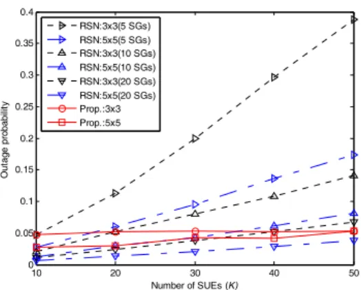
Number of SUEs (K) RSN:3x3(5 SGs)
RSN:5x5(5 SGs) RSN:3x3(10 SGs) RSN:5x5(10 SGs) RSN:3x3(20 SGs) RSN:5x5(20 SGs) Prop.:3x3 Prop.:5x5