Automatic Machine Fault Diagnosis System using Discrete Wavelet Transform and Machine Learning

Automatic Machine Fault Diagnosis System using Discrete Wavelet Transform and Machine Learning

Kyeong-Min Lee

, Caleb Vununu

, Kwang-Seok Moon

, Suk-Hwan Lee

, Ki-Ryong Kwon

ABSTRACT

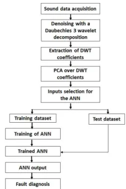
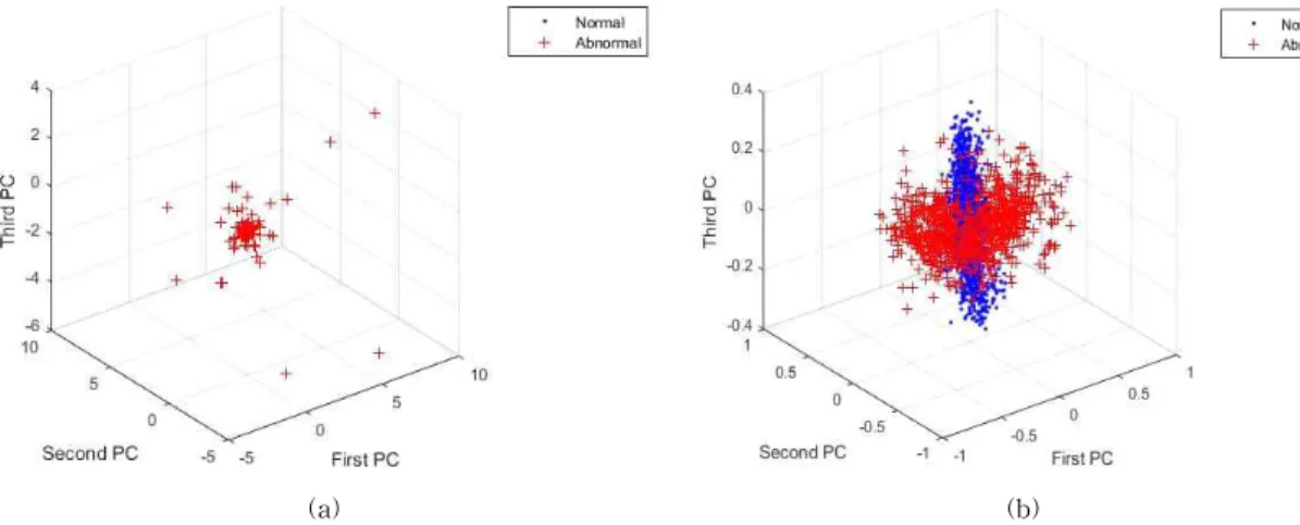
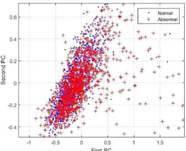
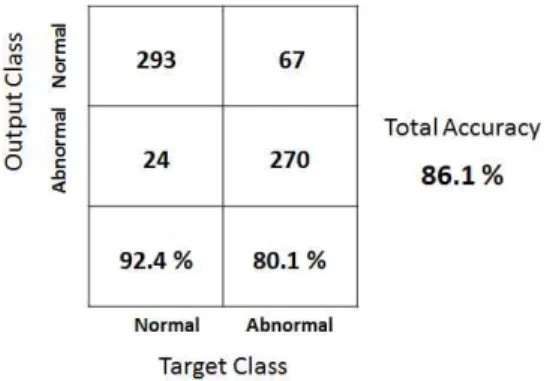
Sounds based machine fault diagnosis recovers all the studies that aim to detect automatically faults or damages on machines using the sounds emitted by these machines. Conventional methods that use mathematical models have been found inaccurate because of the complexity of the industry machinery systems and the obvious existence of nonlinear factors such as noises. Therefore, any fault diagnosis issue can be treated as a pattern recognition problem. We present here an automatic fault diagnosis system of hand drills using discrete wavelet transform (DWT) and pattern recognition techniques such as principal component analysis (PCA) and artificial neural networks (ANN). The diagnosis system consists of three steps. Because of the presence of many noisy patterns in our signals, we first conduct a filtering analysis based on DWT. Second, the wavelet coefficients of the filtered signals are extracted as our features for the pattern recognition part. Third, PCA is performed over the wavelet coefficients in order to reduce the dimensionality of the feature vectors. Finally, the very first principal components are used as the inputs of an ANN based classifier to detect the wear on the drills. The results show that the proposed DWT-PCA-ANN method can be used for the sounds based automated diagnosis system.

Key words: Pattern Recognition, Machine Learning, Machine Fault Diagnosis, Discrete Wavelet Transform, Principal Component Analysis, Artificial Neural Network

※ Corresponding Author : Ki-Ryong Kwon, Address:

(608-737) 599-1, 45 Yongso-ro, Namgu, Busan, Korea, TEL : +82-51-629-6257, FAX : +82-51-629-6230, E-mail : [email protected]

Receipt date : Jun. 21, 2017, Approval date : Aug. 1, 2017

††††

Dept. of IT Convergence and Application Engineering, Pukyong National University

(E-mail : [email protected])

††††

Dept. of IT Convergence and Application Engineering, Pukyong National University

(E-mail : [email protected])

††††

Dept. of Electronics Engineering, Pukyong National University (E-mail : [email protected])

††††

Dept. of Information Security, Tongmyong University (E-mail : [email protected])

†††††

Dept. of IT Convergence and Application Engineering, Pukyong National University

※ This research was supported by Basic Science Research Program through the National Research Foun- dation of Korea (NRF) funded by the Ministry of Science and ICT(No.2016R1D1A3B03931003, No. 2017R1A2B20 12456), ICT R&D program of MSIP/IITP. [2015-0- 00225, Development of Media Application Framework based on Multi-modality which enables Personal Media Reconstruction], and the Pukyong National University Research Park(PK-URP) for Industry-Academic Con- vergence R&D support program in 2017, which is funded by the Busan Metropolitan City, Korea.

1. INTRODUCTION

Among the many problems in industry, the most important factor is for each machine systems to work in a normal state. In order to maintain a nor- mal condition of a machine system, fault prediction and diagnosis systems are necessary. When fail-

ures occur, the failures should be detected as soon

as possible, because if these machines run con-

tinuously under abnormal conditions, it may result

in great damage and even loss of human lives. In

the past, many studies have been based on the tra-

ditional methods of establishing a mathematical

model, analyzing a variety of parameters and then

Fig. 1. Summary of the proposed DWT-PCA-ANN meth- od.

judging the operating conditions of the machine [1].

However, the complexity of the real world machine system and the obvious existence of nonlinear fac- tors such as unwanted noises that can corrupt the used signals make the mathematical models based approaches very difficult to handle and not efficient in terms of accuracy. Since three decades now, machine learning techniques have been widely used in machine fault diagnosis [2-4]. Sounds and vibrations data have shown effectiveness in dam- age detection systems, especially because of their capability of carrying machine operating conditions characteristics. Vibrations and sounds data are in most of studies processed with the same methods for detecting faults.

The authors in [5] reported a detailed review of the different vibration and acoustic methods, such as sound measurements, vibration measurements, the shock pulse method and the acoustic emission technique, for fault diagnosis in rolling bearings.

By just hearing the sound of a machine during its running, an experienced operator can even identify and locate some defined faults in the machine. This shows that the sound signals are strong indicators of the condition of the machine. Compared with vi- brations, sounds can be collected easily by any op- erator who wants to build a diagnosis system, while the sensors that can capture vibrations of the machines are, in practice, difficult to find. That makes the sound-based analysis cheaper and sim- pler to set up while the vibration-based analysis can be expensive and a more complicated task.

Principal component analysis (PCA) [6] is wide- ly used for its capacity of de-correlating data in signal processing. It is also used for the process of dimensionality reduction which is very practical for pattern recognition problems [7]. Artificial Neural Networks (ANN) have shown an im- pressive learning and memory capability. They have been widely used for automatic detection of faults in different ways [8-9]. ANN have the ability to reproduce arbitrary nonlinear functions and are

very suitable for complex pattern recognition tasks [10].

In this research, sound data are collected from healthy and defected drills. We demonstrate here the ineffectiveness of the time domain analysis.

Wavelet transform, instead, allows to conduct a time-frequency domain analysis of the data. Lin [11] demonstrated the effectiveness of wavelet components in fault diagnosis.

In our problem, the collected data being noisy, we first conduct a denoising process using a Daubechies multiple-level wavelet decomposition.

We then extract the wavelet coefficients of the denoised sound signal in order to construct the fea- ture vectors. Each filtered signal is represented by a vector containing its wavelet coefficients. PCA is then performed over the feature vectors in order to reduce their dimensions. The very first principal components are selected and fed to the neural net- work in order to perform the classification task.

The DWT-PCA-ANN proposed method in this

paper is summarized in Fig. 1.

Fig. 2. The 3 steps of the pattern recognition based methods.

2. PATTERN RECOGNITION METHODOLOGY

With all the methods presented above, we can see that pattern recognition techniques comprise three steps: data acquisition, feature extraction and classification. Fig. 2 shows the summary of the pattern recognition methodology. With data ac- quisition, we collect the data that will be processed in order to infer the machine working conditions.

Data acquisition is performed with the material that can allow us to collect the analyzable data. In our case, we have used microphones to collect the sounds of the drills.

Feature extraction is the process of selecting some components of the original data that contain the main characteristics of the elements that we want to analyze. In every pattern recognition prob- lem, the original data must be represented in a short and precise form, so that, the learning algo- rithm can process it easily. Long data can pose ac- curacy problem to the learning algorithm. Here, the goal is not to shorten the data by knowingly ignor- ing whatever can happen later during the process- ing time. But, instead, the goal is to seek for a bet- ter representation that can provide better accuracy.

If the original data can provide a better learning capacity, we can just use it as it was collected. But, if we can shorten the data without degrading the information contained inside it, it is recommended to use the shortened representation, not only for the accuracy facility, but also in order to optimize the processing time. We have used PCA for short- ening our feature vectors composed of wavelet coefficients.

Moreover, as said before, the representation must also be precise. Being short is not the neces- sary and sufficient condition to fulfill. The features must increase the relevancy of the information car-

ried by the data. So, optimizing the processing time during the analysis, and maximizing the relevancy of the information carried by the data are the two main conditions to be fulfilled during the feature extraction process. We demonstrate here that the time series of the sounds do not contain useful in- formation about the damage of the drills, so, they cannot be used as features for our problem. We used the DWT coefficients, instead.

Classification is the last step of the pattern rec- ognition methods. Classification is the fact of cate- gorizing different elements that belong to different instances. In fault diagnosis, classification means the fact of inferring the condition of the machines.

To decide whether the signal comes from a dam- aged or an undamaged machine. The classification method is a learning algorithm that leans from seen data in order to infer the category of the unseen data. After feature extraction process, the selected features will be given to the classifier for the as- sessment of the machines. As said before, the per- formance of the classifier significantly depends on the inputs, which means it depends on the feature extraction process. Because a bad representation of the original data will cause a poor performance, and a good representation will give a successful performance. ANN are used as the classifier in this paper.

3. PRINCIPAL COMPONENT ANALYSIS

PCA [6] is a statistical procedure that uses an

orthogonal transformation in order to convert a set

of correlated data into a set of values that are line-

arly uncorrelated. Those values are called principal

components. The number of the obtained principal

components is less than or equal to the dimension

of the original data. PCA is defined in such a way

that the first principal component has the largest

possible variance, which makes it to be sensitive

to the variability of the dataset. Each succeeding

component in turn must also have the highest var-

iance possible under the constraint that it must be orthogonal to the preceding components. The ob- tained vectors from the principal components will be used as a new basis, called the PCA-space, on which we will project the original data in order to obtain their new representation. That is the part of dimensionality reduction capability of the PCA.

The PCA de-correlates the data. Which means that it forces the uncorrelated data in the dataset to be separated. Because of that, after the projec- tion on the PCA-space, the set of data that are highly correlated between them will be put togeth- er in one cluster. Data that are not correlated at all between them will be separated. Therefore, PCA allows to investigate the variance of a dataset.

4. ARTIFICIAL NEURAL NETWORK

Artificial neural network (ANN) is an inter- connected group of artificial neurons. These neu- rons use a mathematical or computational model for information processing. ANN is an adaptive system that changes its structure based on in- formation that flows through the network [12]. The neural network acquires the ability to generalize based on the training data and, if the training data contains all the characteristics, all the meaningful information possible of the processed sounds or vi- brations, the network can predict outcomes for new, previously unseen data sound or vibrations.

One of the commonly used structures of ANN is the multi-layer perceptron. Using supervised learning, the sample {x

} is fed to the network and produces an output {y}.

The input pattern {x

} is then propagated through the network in the following way:

(1)

Where y

denotes the output of a given neuron i, and N the number of input neurons, while M de- notes the number of hidden layers. is the

weighted sum in this form: j represents the input neuron that comes to feed the neuron, and n de- notes the layer where we are (n = 1 represents the first layer). To implement this procedure, one needs to calculate the error derivative with respect to weight in order to change the weight by an amount that is proportional to the rate at which the error changes as the weight is changed. The backpropagation algorithm [12] is used in this re- search paper. The activation function f is a sigmoid function (see figure 4) and is defined as:

(2)

5. WAVELET BASED DENOISING AND FEATURE EXTRACTION

The sounds data are extremely disturbed by the environment-related noises. Those noises can be the sounds generated by other machines in the in- dustry site or even the sounds that can come from the operators located in the site. The background noise of the experimental site was not measured in our work. The two machine condition states that we want to detect, the normal and abnormal con- ditions, are different intrinsically. But, the complex nature of the environment of the machinery system makes the collected data sounds from healthy and faulty drills really noisy, very similar and very much difficult to distinguish or to separate. Fig. 3 shows the plot of the data sounds with the PCA analysis using their time series components. As we can see, the normal and abnormal data are not distinguishable. Unlike in [13], where the used data were highly separable, in the present work, the ob- tained data are pretty much identical, they are all mixed together as if they were belonging to the same dataset, as we can see in figure 3. Using the time series based methods proposed in [13] and [14]

is ineffective because the time series components

of these data do not contain any useful information

concerning the health state of the drills. All the

purpose of the new feature extraction method pro-

Fig. 3. Normal and abnormal data sounds using their time series.

(a) (b)

(c) (d)

Fig. 4. Sound signals and their corresponding power spectral density function: (a) normal sound, (b) abnormal sound, (c) power spectral density of normal sound, and (d) power spectral density of abnormal sound.

posed in this work is to find the existing differ- ences between the normal and abnormal sounds in order to recognize them automatically.

The high frequencies of the sounds are related to the noise. The idea is to de-noise the signals using a low-pass filter with an appropriate cutoff frequency. The sounds from both drills being ex- tremely similar because of noises, using the fre- quencies where most of the energy of signal is lo- cated does not help to make a difference between the normal and the abnormal data. In figure 4, we can see that most of the energy is located between around 1000 Hz and around 5000 Hz for the normal data and between 3000 Hz and 6500 Hz for the ab- normal data sound. We have first filtered each data using a bandpass filter according to the region where the energy is mostly concentrated. And then, we have conducted a PCA-based similarity analysis between the obtained filtered normal and abnormal data (results are shown in figure 5).

With a quick visual inspection of figure 5, we

Fig. 5. Normal and abnormal data sounds after filtering using the frequencies where the maximal energy is located.

Fig. 6. Multiple-level decomposition of DWT. Each cA

represents the approximation (A) and its corre- sponding coefficients at level j. Each cD

repre- sents the details (D) and its corresponding co- efficients at level j.

see that, using the location where the concentration of the energy is maximal does not capture the dif- ferences between the normal and the abnormal sounds. The data remain identical, just like the ones showed in figure 3. Therefore, we propose to remove all the high frequencies of the data and re- tain only the frequencies around 5000 Hz. In this purpose, we can use the DWT based multiple-level decomposition that allows the filtering in the low frequencies. The DWT decomposition at the level 3 represents a low-pass filtering with cutoff fre- quency at around 5512.5 Hz. We can perform a

Daubechies wavelet transform at level 3 in this purpose. Fig. 6 represents graphically the process of denoising.

Using the wavelet decomposition, the low fre- quency and the high frequency components are ex- tracted at each level. The extracted low-frequen- cies are then used to approximate the denoised version of the signal using the wavelet coefficients obtained from the first decomposition. The newly created signal is then decomposed at the next level where the high frequency components are removed again and the new wavelet coefficients will be used to approximate a more denoised version of the signal. The newly denoised version will be decom- posed again. And so on, we can go through each level by removing most of the high frequency components.

In figure 6, S represents the original signal. The first decomposition is performed using low-pass and high-pass filters simultaneously. The co- efficients obtained from the low-pass filtering are called the approximation (cA

) and those obtained from the high-pass filtering are called the details (cD

). The cA

coefficients will be used to obtain the denoised version S' of the original signal S by reverting the wavelet decomposition. A second de- composition, which means, the second level de- composition, can be performed using the same process (low-pass and high-pass filtering simul- taneously) over the denoised signal S'. Then, the obtained approximation cA

from S' will be used to get a more denoised version of S, the signal S''.

The same process can be conducted until we get the denoised version of S that we want. In our work, we seek for a denoised version that contains the frequency elements around the 5000 Hz.

In figure 7, we can see the denoised version of the two signals and their corresponding power spectral density functions. We can see that all the high-frequency components are removed and the retained frequency elements are below 5000 Hz.

The maximum energy of the filtered signals is lo-

(a) (b)

(c) (d)

(e) (f)

Fig. 7. Sound signals, their filtered versions and the power spectral density function of the filtered versions: in the left (a, c, and e) we have the normal sound, in the right (b, d, and f) the abnormal signal.

cated around 1000 Hz and 4000 Hz for the normal signal and between 0 Hz and 4000 Hz for the ab- normal data sound. The DWT coefficients of these denoised signals will be extracted in order to be used as the features of the fault condition. The re- sults using this denoising method and the corre- sponding DWT coefficients as features are dis-

cussed in section 7.

6. EXPERIMENTAL SETUP AND DATA ACQUISITION

We want to detect defected drill by analyzing

the sounds emitted by it during its operating time.

(a) (b)

Fig. 8. Comparison between the PCA results of: the time series data (a) and the DWT coefficients of the denoised version of the signals (b) using only the first two principal components.

We have collected data sounds from an undamaged and a damaged drill using a microphone. We put the undamaged drill in the cutting machine then we’ve recorded the sounds for one minute and half.

Then, we take out the undamaged drill, replace it by the damaged one. We’ve recorded the sounds from both the undamaged drill and the damaged one. Sound being a nonstationary data, we’ve seg- mented the recorded sound into many parts to con- struct our dataset for the pattern recognition. The sampling frequency used was 44100 Hz and the signal length was 50 ms (0.05 s). We have created a dataset of 2183 data sounds, 1120 from the un- damaged drill and 1063 data from the damaged drill. We can see some samples from our dataset in the figures 4 and 7.

7. RESULTS AND DISCUSSION

We have started by extracting the wavelet co- efficients of the denoised versions of our data.

Then, we applied PCA on the newly created feature vectors containing the wavelet coefficients. The result is shown in figure 8. We can see that the time series do not contain any useful information that can be used for the purpose of diagnosis. The two datasets, using their time series, are highly correlated, that is why the PCA outputs all of these

data extremely close between them. But, using the discrete wavelet coefficients, we can see that the normal and abnormal data become separable. In figure 8 (b), we see that most of the normal data remain confined around the origin of the PCA- space while the abnormal data are spread all around the origin. This is because there are now strong variations between the two new datasets created with the DWT coefficients.

The abnormal data sounds are scattered all over the PCA-space. Two main reasons for that: first, the sounds emitted by the damaged drill are much noisier than the ones generated by the healthy drill.

Second, they are pretty unstable over time. That makes the variance of the abnormal dataset very significant compared to the variance of the normal dataset whose data appear to be very much stable over the time. That stability makes the normal data to be confined around the origin of the PCA-space.

The denoising process significantly increases the variance, which means the differences, between the two datasets. Their differences become much clearer in figure 8 (b) than in figure 8 (a).

The denoised versions of the signals are

different. Using the data in figure 8 (a), there is

no classifier that can separate well these data. The

results of the neural network using the data in fig-

ure 8 (a) were really poor. But, the data in figure

(a) (b)

Fig. 9. Comparison between the PCA results of: the time series data (a) and the DWT coefficients of the denoised version of the signals (b) using the first three principal components.

Fig. 10. Confusion matrix of the testing data.

8 (b) become different after the denoising process.

Any nonlinear classifier can separate those data.

An even better representation of the “separabil- ity” (the fact that the data can easily be separated by any nonlinear classifier) can be seen if we use up to three principal components to project the original data. Fig. 9 shows the result of using the first three principal components. Because the first components contain all the useful information of the dataset, a few number of principal components will be later selected for feeding the classifier.

We can see from figure 9 that the time series data, even using the three PC-projection still can- not make the data separable. A quick look to the figure 9 (a) shows that all the data, normal and abnormal, are mixed together in one cluster, in one class, the normal data even being nonvisible in the figure because they are all confined around the origin. But, in 9 (b), we clearly distinguish two dif- ferent clusters. One cluster, in the middle, repre- sents the normal data and the other cluster, sur- rounding the first data, represents the abnormal dataset.

We have selected the first twenty principal com- ponents for feeding our neural network. Which means that our network will have 20 inputs neurons. The network has 3 layers. The input layer has 20 neurons, the hidden layer has 10 neurons

and the last layer has 2 neurons for our 2 instances (normal and abnormal). The learning function used in the network is described in equation (2). The results are shown in figure 10.

As said before, we have collected 2183 data dur- ing the data acquisition process. 1120 normal and 1063 abnormal data. 70% of each dataset was used for training and the remaining 30% was used for testing.

Normal dataset: 1120 data, 790 were used for training and 330 for testing. 322 data out of 330 were classified as normal and only 8 data were misclassified, as shown in Figure 10. That gives an accuracy of 97.5 % over the unseen data.

Abnormal dataset: 1063 data, 739 were used for

training and 324 for testing. 304 data out of 324

were classified as abnormal. 20 data sounds were

Fig. 11. Confusion matrix of the testing data using the PCA over the time series data.

Fig. 12. Normal and abnormal data sounds using their time series based statistical features.

misclassified. This is explained by the fact that the abnormal data, as discussed previously in this sec- tion, are well unstable over time. As described in section 6, we have recorded the sounds from both drills and then segmented it into many parts in or- der to build the dataset. The instability of the ab- normal data comes from the fact that the faulty drill can sometimes, although rarely, produce sounds that appear to be similar to the sounds pro- duced by the healthy drill. Despite that instability, the proposed method allows to achieve a good performance. With only 20 abnormal data being misclassified, the network achieves an accuracy of 93.8 %.

The total accuracy of the classifier is 95.7 % (see Fig. 10).

We have conducted a comparative study with the time series based methods developed in [13]

and [14]. In the present paper, we have demon- strated the feasibility of a DWT-PCA-ANN meth- od, using the discrete wavelet coefficients as the features, then using the principal component anal- ysis for the dimensionality reduction and then an artificial neural network based classifier. We have demonstrated in the same time the ineffectiveness of using the time series of the data sounds. In [13]

and [14] instead, the authors have adopted the time series based analysis, computing the principal components [13] or the statistical features [14].

Using the vibration signals of ball bearing compo- nents, the authors in [14] have computed for each signal 6 statistical features (the range, the mean value, the standard deviation, the skewness, the kurtosis, and the crest factor) that have been used as the inputs of the neural network.

Firstly, we have performed the PCA over our dataset using the time series. The first five princi- pal components were selected and fed to a neural network based classifier, as proposed in [13]. The network’s architecture remains the same, as used in [13], which means that the input layer has 5 neu- rons, the hidden layer has 10 neurons and 2 neu-

rons for the output layer. The results using this method are shown in figure 11. As we can clearly see, the performance of the network is really poor.

We must recall that the data used for this method are the ones shown in figure 3. Any nonlinear clas- sifier will be unable to separate those data. Espe- cially for the abnormal dataset, the network ach- ieves a deceiving 46.1 % accuracy by misclassify- ing 181 data of the 336 testing data.

Secondly, for each data sound in the dataset, we

have computed the six statistical features pre-

sented above and used them as the inputs of a three

layers neural network, as proposed in [14]. The in-

puts layer has 6 neurons, the hidden layer 10 and

the output layer 2. We have plotted all the data rep-

resented by their statistical features in figure 12

Table 1. Results summary

C. Vununu et al. [13] P.K. Kankar et al. [14] Present work Feature Extraction

Method Time series + PCA Time series + statistical

features DWT coefficients + PCA

Classifier Neural network Neural network Neural network

Accuracy 62.8 % 86.1 % 95.7 %

and we can see that they remain relatively identical.

The results of the classification using these data are shown in figure 13. Here, the network increases the accuracy, but still remains poor, compared to our proposed method. In total, 91 data over the 654 were misclassified (86.1 % of accuracy, see figure 13), while for our method, only 28 data were mis- classified.

Fig. 13. Confusion matrix of the testing data using stat- istical features as feature extraction.

In Table 1 below, we made a summary of the results of the 3 methods.

8. CONCLUSION

The DWT-PCA-ANN method proposed in this study proves that it can reach outstanding per- formance in pattern recognition based fault diag- nosis of drills using sounds. We’ve used PCA over the DWT coefficients of the denoised versions of the signals, then we’ve selected the first five prin- cipal components as the inputs of our neural net- work based classifier. And the method shows that it can have a very good performance. Compared

to the time series analysis, DWT coefficients pro- vide better information of the faults of the drills.

The time series analysis could not reach a 70% of accuracy.

The DWT-PCA-ANN method can be used in any other fault diagnosis system. If it can separate normal and abnormal sounds of the drills, it can be also used for vibrations and other acoustic emission data.

REFERENCE

[ 1 ] M.M. Polycarpou and A.T. Vemuri, “Learning Methodology for Failure Detection and Accommodation,” IEEE Control Systems, Vol. 15, Issue 3, pp. 16-24, 1995.

[ 2 ] N.R. Sakthivel, V. Sugumaran, and B.B. Nair,

“Application of Support Vector Machine (SVM) and Proximal Support Vector Machine (PSVM) for Fault Classification of Mono Block Centrifugal Pump,” International J ournal of Data Analysis Techniques and Strategies, Vol. 2, No. 1, pp. 38-61, 2010.

[ 3 ] Y. Xu and H. Wang, “A New Feature Selec- tion Method Based on Support Vector Machines for Text Categorization,” Interna- tional J ournal of Data Analysis Techniques and Strategies, Vol. 3, No. 1, pp. 1-20, 2011.

[ 4 ] N.R. Sakthivel, B.B. Nair, V. Sugumaran, and

R.S. Rai, “Application of Standalone System

and Hybrid System for Fault Diagnosis of

Centrifugal Pump Using Time Domain

Signals and Statistical Features,” International

Journal of Data Mining Modeling and

Management, Vol. 4, No. 1, pp. 74-104, 2012.

[ 5 ] N. Tandon and B.C. Nakra, “Vibration and Acoustic Monitoring Techniques for the De- tection of Defects in Rolling Element Bearings -A Review,” The Shock and Vibration Digest, Vol. 24, No. 3, pp. 3-11, 1992.

[ 6 ] K. Pearson, “On Lines and Planes of Closest Fit to Systems of Points in Space,” Philo- sophical Magazine Series 6, Vol. 2, Issue 11, pp. 559-572, 1901.

[ 7 ] V. Emamian, M. Kaveh, A.H. Tewfik, Z. Shi, L.J. Jacobs, and J. Jarzynski, “Robust Cluster- ing of Acoustic Emission Signals Using Neural Networks and Signal Subspace Pro- jections,” EURASIP Journal on Advances in Signal P rocessing, No. 3, pp. 276-286, 2003.

[ 8 ] M. Subrahmanyam and C. Sujatha, “Using Neural Networks for the Diagnosis of Local- ized Defects in Ball Bearings,” Tribology International, Vol. 30, No. 10, pp. 739-752, 1997.

[ 9 ] B. Samanta, K.R. Al-Balushi, and S.A. Al- Araimi, “Artificial Neural Networks and Support Vector Machines with Genetic Algorithm for Bearing Fault Detection,” Engineering Appli-

cations of Artificial Intelligence, Vol. 16, No.

7-8, pp. 657-665, 2003.

[10] R.O. Duda, P.E. Hart, and D.G. Stork, Pattern Classification, Wiley, New York, 2001.

[11] J. Lin, “Feature Extraction of Machine Sound Using Wavelet and Its Application in Fault Diagnosis,” NDT and E International, Vol. 34, Issue 1, pp. 25-30, 2001.

[12] D.E. Rumelhart, G.E. Hinton, and R.J. Wil- liams, “Learning Representations by Back- Propagating Errors,” Nature, Vol. 323, pp.

533-536, 1986.

[13] C. Vununu, J.H Park, S.H. Lee, K.R. Kwon,

“Sound Based Machine Fault Diagnosis Sys- tem Using Pattern Recognition Techniques,”

Journal of Korea Multimedia Society, Vol. 20, No. 2, pp. 134-143, 2017.

[14] P.K. Kankar, Satish C. Sharma, and S.P.

Harsha, “Fault Diagnosis of Ball Bearings

Using Machine Learning Methods,” Expert

Systems with Applications, Vol. 38, Issue 3,

pp. 1876-1886, 2011.

Kyeong-Min Lee

She received a B.S. degree in Computer Engineering in Dong- eui University, Korea in 2000.

She received a M.S degree in Electronics Engineering in Donga University, Korea in 2002. She is currently a Ph.D. in department of IT Convergence and Application engineering at the Pukyong National University. Her research interests include signal processing, digital image processing, and machine learning.

Caleb Vununu

He received his B.S. degree in Computer Science in Youngsan University, Republic of Korea in 2015. Since September 2015, he is a Master degree student in the department of IT Convert- gence and Application Engin- eering in Pukyong National University. His research interests include signal processing and machine learning.

Kwang-Seok Moon He received the B.S., or Studies M.S., and Ph.D degrees in Elec- tronics Engineering in Kyung- pook National University, Korea in 1979, 1981, and 1989 respec- tively. He is currently a professor in department of Electronic en- gineering at Pukyong National University. His re- search interests include digital image processing, video watermarking, and multimedia communication.

Suk-Hwan Lee

He received a B.S., a M.S., and a Ph. D. degrees in Electrical Engineering from Kyungpook National University, Korea in 1999, 2001, and 2004 respec- tively. He is currently an asso- ciate professor in Department of Information Security at Tongmyong University. His research interests include multimedia security, digital image processing, and computer graphics.

Ki-Ryong Kwon

He received the B.S., M.S., and

Ph.D. degrees in electronics en-

gineering from Kyungpook Na-

tional University in 1986, 1990,

and 1994 respectively. He work-

ed at Hyundai Motor Company

from 1986-1988 and at Pusan

University of Foreign Language from 1996-2006. He

is currently a professor in Department of IT Convert-

gence and Application Engineering at the Pukyong

National University. He has researched University of

Minnesota in USA in 2000-2002 with Post-Doc. and

Colorado State University on 2011-2012 with visiting

professor. He was the President of Korea Multimedia

Society in 2015-2016. His research interests are in the

area of digital image processing, multimedia security

and watermarking, bioinformatics, weather radar in-

formation processing, and machine learning.