1. Introduction
Forest with high ratio of coniferous trees consists of 64 % of Korean territory and this property makes the land vulnerable to forest disaster(Byun, 2014).
Yangyang-gun, Gangwon-do which has superiority of coniferous trees represents a vegetation characteristic of Korea. A damaged area from a forest fire which occurred in 2005 at Yangyang-gun was mostly comprised of pine forest(Kyosu newspaper, 2005). To prevent further damages over the area local authorities decided to plant deciduous trees which have fire-resistant properties. This decision gave the researcher an responsibilities to monitor the area using the state-of-art technology.
Generally there are two techniques used for monitoring vegetation; field surveying and remote sensing method. Field surveying can be an appropriate method to monitor the small details about the condition of vegetation but its application is limited when applying to the extensive areas and when obtaining time series data from the past.
Remote sensing technique, on the other hand, is widely used to monitor the wide and unaccessible areas. It also provides useful information of the past if satellite imagery has been acquired periodically.
Landsat series, for example, first launched in 1972 have provided not only extensive coverage but also have extensively acquired many imagery over the same site. In addition with its capability to acquire
Received: 2016.05.27, revised: 2016.06.14, accepted: 2016.11.10
* Member, M. S. Student, School of Civil & Environment Engineering, Yonsei University, [email protected]
** Member, Staff, Korea Land and Geospatial Informatix Corperation, [email protected]
*** Member, Ph. D. Student, School of Civil & Environmental Engineering, Yonsei University, [email protected]
**** M. S. Student, School of Civil & Environmental Engineering, Yonsei University, [email protected]
***** Corresponding Author, Member, Professor, School of Civil & Environmental Engineering, Yonsei University, [email protected]
Analysis of Changes in NDVI Annual Cycle Models Caused by Forest Fire in Yangyang-gun, Gangwon-do Using Time Series of Landsat
Images
*
Choi, Yoon Jo*ㆍCho, Han Jin**ㆍHong, Seung Hwan***ㆍLee, Su Jin****ㆍ Sohn, Hong Gyoo*****
Abstract
Sixty four percent of Korean territory consists of forest which is fragile for forest fire. However, it is difficult to detect the disaster-induced damages due to topographic complexity in mountainous areas and harsh weather conditions. For this reason, satellite imaging systems have been widely utilized to detect the damage caused by forest fire. In particular, ground vegetation condition can be estimated from multi-spectral satellite images and change detection technique has been used to detect forest fire damages. However, since Korea has clear four seasons, simple change detection technique has limitation. In this regard, this study applied the NDVI(normalized difference vegetation index) annual cycle modeling technique on time-series of Landsat images from 1991 to 2007 to analyze influence of forest fire of Yangyang-gun, Gangwon-do in 2005 on vegetation condition. The encouraging result was obtained when comparing the areas where forest fire occurs with non-damaged areas. The mean value of NDVI was decreased by 0.07 before and after the forest fire. On the other hand, annual variability of NDVI had been increasing and peak value of NDVI was stationary after the forest fire. It is interpreted that understory vegetation was seriously damaged from the forest fire occurred in 2005.
Keywords : Forest Fire, Landsat TM, NDVI, Annual Cycle Model
3 (Journal of the Korean Society for Geospatial Information Science) Vol.24 No.4 December 2016 pp.3-11
연구논문
ISSN: 2287-6693(Online) http://dx.doi.org/10.7319/kogsis.2016.24.4.003
the imagery using multi-spectral bands, Landsat series have been widely used in the science community because the images are free to the general public since 2008.
Many studies related to the vegetation condition have been done in the field of drought monitoring, forest fire identification, agricultural productivity estimation, and vegetation regeneration monitoring (Labus et al., 2002; Peters et al., 2002; van Leeuwen, 2008; Vila et al., 2010). However, in most of these studies, vegetation conditions of a certain period have been represented by some indicies in an individual satellite image. Accordingly, analysis of forest fire effect has been usually conducted based on the indices extracted from an individual image. However, since Korea has distinctive seasons, the characteristic of satellite imagery which has a periodicity is limited to analyze vegetation variability. To overcome these barriers, a technique which could reflect a continuity of vegetation cover is critical. Beck et al.(2006) developed a double logistic function model to describe NDVI(normalized difference vegetation index) time series in high-latitude environments.
Verbesselt et al.(2010) presented a generic approach for detection and characterization of change in time series, which can robustly detect change. Jung et al.
(2013) proposed harmonic model to characterize patterns of variation in MODIS NDVI time series data from 2006 to 2012. But when the change of data vary greatly it is difficult to apply this model.
Temperature is a primary factor affecting the rate of plant development(Hatfield and Prueger, 2015). Ha et al.(2007) also demonstrated that vegetation condition is closely related with average temperature.
Bechtel(2012) proposed annual temperature cycle model which is approximated with a constant term plus sine function to characterize the annual cycle of land surface temperature with Landsat archives. Hong et al.(2015) applied annual temperature cycle model proposed by Bechtel(2012) to identify the variation of temperature inside the city. And they proved that the model fitted well in South Korea.
In this study, we extended the annual temperature cycle model to analyze vegetation variability before and after a forest fire. Yangyang-gun, Gangwon-do
was selected as an experiment site where big forest fire had frequently occurred since 1960(Lee et al., 2012). To analyze the influence of forest fire on the model parameters, nine AOIs(area of interest) were set as forest fire-affected area, area nearby the forest and mountainous area. To improve precision of the model, effects of clouds and cloud shadows were excluded by using Fmask(function of mask) algorithm and then outliers were removed by RIRLS-based(robust iteratively reweighted least squares) filtering technique. After investigating the NDVI trend using the NDVI annual cycle model, the seasonal changes of NDVI values using single Landsat images were analyzed and compared with the results of NDVI annual cycle modeling.
2. Study Site and Materials 2.1 Study Site
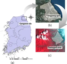
The study site locates in Yangyang-gun, Gangwon- do. A severe forest fire had occurred for 32 hours from April 4 to 6, 2005. Approximately 973 hectares of forest and Naksansa Temple were affected by the forest fire. Study area covers approximately 212,095,800
including both forest fire-affected area and non-affected area. Fig. 1 shows location of our study area and Fig. 2 shows the location of AOIs
Figure 1. Location of study area: (a) Gangwon-do, (b)
Yangyang-gun, (c) forest fire-damaged areas
(2005/05/30)
Series of Landsat Images 5
Figure 2. Location of AOIs
to identify the influence of forest fire on the NDVI annual cycle model.
In Fig. 2, the areas of 1, 2, and 3 indicate the areas affected by the forest fire, 4 and 5 the areas nearby the forest fire events, and 6, 7, 8, and 9 the mountainous areas, respectively.
2.2 Satellite Imagery
In this study, we used series of Landsat TM images. For maintaining consistency, Landsat ETM+
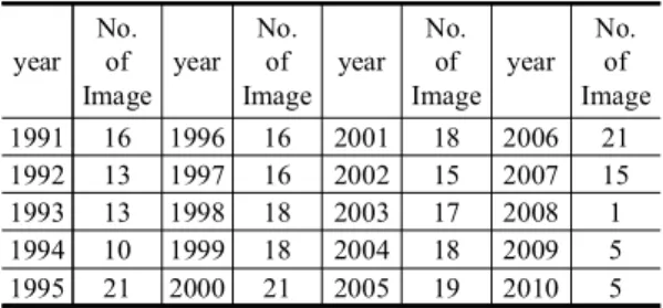
and OLI were not used in this study. Table 1 shows the numbers of Landsat TM scenes covering the study site. There were total 296 images available from 1991 to 2010. However, as shown in Table 1, the number of Landsat images after 2008 was not sufficient to apply the trend analysis of vegetation.
Therefore, we performed the trend analysis only using 285 images obtained from 1991 to 2007 over the study areas.
year No.
of Image
year No.
of Image
year No.
of Image
year No.
of Image
1991 16 1996 16 2001 18 2006 21
1992 13 1997 16 2002 15 2007 15
1993 13 1998 18 2003 17 2008 1
1994 10 1999 18 2004 18 2009 5
1995 21 2000 21 2005 19 2010 5
Table 1. Number of Landsat TM images capturing Yangyang-gun, Gangwon-do from 1991 to 2010
3. Satellite Image Processing 3.1 Image Preprocessing
Since Landsat data are provided as DN(digital number) images with a range between 0 and 255, it is required to convert DN value into reflectance value(
) when performing the land surface analysis.
In this study, the algorithms proposed by Chander and Markham(2003) and NASA(2013) were applied to convert DN values into reflectance values. When multiple images are used, the effect caused by different solar zenith angles and the exoatmospheric solar irradiances can be compensated by converting original pixel values into reflectance(Chander and Markham, 2003). The formulas used for the conversion are listed in Eqs. (1) and (2).
∙ (1)
∙cos
∙
∙
(2) where,
: radiance at the sensor’s aperture
∙
∙
: original pixel value
: gain value for a specific band
: bias value for a specific band
: unitless planetary reflectance
: Earth-Sun distance in astronomical units
: mean solar exoatmospheric irradiance
: solar zenith angle
3.2 Noise Filtering
Since Landsat TM image typically includes cloud
and cloud shadow pixels, they could make
observation impossible and have an influence on the
results of ground condition analysis. To release the
influence of cloud and cloud shadow pixels, it is
required to remove the cloud and cloud shadow
pixels before the actual analysis. In this study, the
noise filtering algorithm proposed by Zhu and
Woodcock(2012) was applied. This algorithm can
easily detect pixels of clouds and cloud shadows with
high accuracy. The algorithm was conducted in two
steps. In its first step the object-based technique for classifying cloud and cloud shadow pixels is performed. The technique is called Fmask algorithm.
Since the areas covered by clouds and cloud shadows present lower temperature than other areas, the shadow pixels can be extracted using the thermal infrared band information of Landsat image(Vermote and Saleous, 2007). After this, clouds and cloud shadows were matched based on the similarity of objects and sun angle.
Almost all cloud and cloud shadow pixels can be removed by Fmask, but some noise pixels might still remain. To remove the noise pixels and minimize the distortion caused by the noise pixels, RIRLS model was additionally adopted after performing the Fmask algorithm(Street et al., 1988; O’Leary, 1990; Zhu et al., 2012; Zhu and Woodcock, 2014). The pixels having lower or higher values than the matched value in the RIRLS model were filtered out by considering them as outliers. RIRLS model can be represented by Eq. (3).
cos
sin
cos
sin
(3)
Where,
: Julian date
: number of days per year (T= 365)
: number of years of Landsat data
: coefficient for overall values for NDVI
: coefficients for intra-annual change for NDVI
: coefficients for inter-annual change for NDVI
: predicted value for the NDVI at Julian date x based on RIRLS fitting.
3.3 NDVI Calculation
The Landsat TM imagery consists of 7 spectral bands. From the multi-spectral imagery, the indices which represents ground condition can be computed with a combination of these bands. NDVI is the most powerful index to analyze the traits of vegetation.
The NDVI is computed by the reflectance values of the near infrared band(
; band 4) and red band (
; band 3) on Landsat TM image. The formula to calculate NDVI is Eq. (4).
(4)
3.4 NDVI Annual Cycle Model
Since ground vegetation condition generally follows annual variation trends, the methodology which can reflect continuity is required. Bechtel (2012) proposed annual temperature cycle model defined by sine function to characterize the annual cycle of land surface temperature with time series of Landsat images. To analyze the vegetation variability, this paper proposes annual NDVI cycle model applying annual temperature cycle model proposed by Bechtel(2012) using a time series of Landsat images. Annual cycle model is modelled with sine function and can be represented by Eq. (5).
∙sin
(5) Where,
: annual cycle model
: mean of NDVI
: amplitude of the annual NDVI cycle
: optional phase shift from the equinox
: day of the cycle
, and of Eq. (5) were estimated by an unconstrained nonlinear optimization algorithm, which minimizes the square sum of the residuals (Bechtel, 2012).
4. Results 4.1 Noise Filtering
Fig. 3 shows Landsat TM image on May 14, 2005
and detected cloud and cloud shadow pixels in the
image after applying the Fmask algorithm. As shown
in Fig. 3(b), cloud and cloud shadow pixels were
extracted.
Series of Landsat Images 7
(a) (b)
Figure 3. Results of applying Fmask: (a) Landsat imagery (2005/5/14), (b) cloud and cloud shadow pixels extracted from Landsat imagery by Fmask (white: cloud, gray:
cloud shadow)
Number of images Before
filtering
After Fmask filtering
After RIRLS filtering AOI #1
285
147 107
AOI #2 156 116
AOI #3 152 115
AOI #4 146 99
AOI #5 147 108
AOI #6 140 97
AOI #7 153 108
AOI #8 148 107
AOI #9 149 105
Table 2. Results of Fmask and RIRLS filtering
In order to create a stable annual cycle model, the remained noise pixels after applying Fmask were filtered out by RIRLS model. Forest fire caused significant changes on the vegetation conditions. For this reason, NDVI annual cycle modeling was conducted separately before and after on April 4, 2005, the day when a huge forest fire occurred.
Table 2 summarized the number of available images in each of the AOI after applying Fmask algorithm and RIRLS-based filtering technique. As shown in Table 2, about 97~116 scenes in each AOI after filtering were available among total 285 Landsat images. In other words, 59~66% of total images we used were filtered out in the final stage.
4.2 NDVI Annual Cycle Models
From the Landsat images of which pixels of cloud and cloud shadow were removed, NDVI annual cycle model of each AOI were calculated. Fig. 4 shows the results of the annual cycle modeling. As shown in Fig. 4, the seasonal variation of NDVI were identified and the NDVI values of each AOI were fitted to an annual cycle model. In particular, as shown in Figs. 4(a), 4(b) and 4(c), the annual cycle models of AOIs #1 to #3 where forest fire occurred were changed. Moreover, while AOIs #4 to #5
AOI Change Mean Amplitude Shift
Affected area
AOI #1 Before forest fire 0.4165 0.1668 0.9640
After forest fire 0.3448 0.2420 0.8439
AOI #2 Before forest fire 0.3817 0.1621 0.7641
After forest fire 0.3011 0.2500 0.7267
AOI #3 Before forest fire 0.3884 0.1620 0.7965
After forest fire 0.3135 0.2361 0.7511
Nearby area
AOI #4 Before forest fire 0.4300 0.1701 0.8758
After forest fire 0.4198 0.2178 0.8906
AOI #5 Before forest fire 0.4110 0.1596 0.7869
After forest fire 0.3935 0.2144 0.8500
Mountainous area
AOI #6 Before forest fire 0.4184 0.3087 0.9648
After forest fire 0.4743 0.3012 1.1825
AOI #7 Before forest fire 0.4311 0.3113 1.0424
After forest fire 0.4578 0.3004 1.1090
AOI #8 Before forest fire 0.4231 0.3210 0.9883
After forest fire 0.4482 0.2935 1.1496
AOI #9 Before forest fire 0.4441 0.2696 0.9773
After forest fire 0.4771 0.2592 1.0935
Table 3. Changes in annual NDVI cycle models before and after forest fire in 2005
Figure 4. Annual NDVI cycle model of each AOI: (a) to (c) AOIs damaged by forest fire, (d) to (e)
AOIs nearby forest fire-damaged areas, (f) to (i) AOIs in mountainous areas
Series of Landsat Images 9
showed similar trends before and after the forest fire, the NDVI mean values in AOIs #1 to #3 dropped sharply about 0.07 after the forest fire. Meanwhile, NDVI mean values in AOIs #4 to #5 decreased about 0.02 and AOIs #7 to #9 increased about 0.03. The change of NDVI mean values in AOIs #4 to #5 displayed the insensible change but both areas showed a decreasing tendency. As both areas are the forest fire nearby area, it might be affected by the forest fire.
Amplitude of the annual NDVI cycle showed an increasing tendency of the forest fire-affected areas and nearby areas after the forest fire. In particular, the peak values of NDVI in Fig. 4 were stable even after forest fire. The reason why NDVI peak values were not much changed after the forest fire is that it might be influenced by reforestation program such as
‘Forest restoration plan at Yangyang special disaster district’ and ‘Forest management development project at major landscape area’(Korea Forest Service, 2013).
On the other hand, the NDVI trough values in Fig.
4 were distinctly decreased after the forest fire. It was because the NDVI trough values generally present vegetation condition in winter seasons and
the influence of the upper layer of trees is excluded.
Therefore, the results demonstrated that the understory vegetation became bare soil after the forest fire.
At the mountainous areas, mean and amplitude values of the annual NDVI cycle are larger than those of the other areas. For AOIs #6 to #9, NDVI mean values increased by 0.02 and amplitude of annual cycle decreased by 0.01 after the forest fire.
It is opposite trend with other areas, in which showed decreasing trend in mean values of NDVI and increasing trend in amplitude. The change of vegetation variability was insignificant and consistent tendency was observed.
On the other hand, the difference of the phase shift values before and after the forest fire was not significant because of the low spatial variability. The results implied that there was scanline error and time interval of the images was not too long to have influence on annual cycle model (Bechtel, 2012;
Hong et al., 2015).
4.3 Single Imagery Analysis
To confirm the change tendency resulted from
AOI Change January
2004-2010
May 2003-2009
August 2004-2007
November 2003-2005
Affected area
AOI #1 Before forest fire 0.2777 0.4340 0.6310 0.3735
After forest fire 0.2683 0.5424 0.6318 0.3203
AOI #2 Before forest fire 0.2948 0.3578 0.6219 0.3541
After forest fire 0.2118 0.4706 0.6078 0.2341
AOI #3 Before forest fire 0.2510 0.3092 0.5231 0.3114
After forest fire 0.2175 0.4132 0.5262 0.2627
Nearby area
AOI #4 Before forest fire 0.1501 0.1894 0.2611 0.1685
After forest fire 0.1540 0.2227 0.2636 0.1869
AOI #5 Before forest fire 0.1478 0.1740 0.2817 0.1711
After forest fire 0.1681 0.2295 0.2846 0.1967
Mountainous area
AOI #6 Before forest fire 0.1130 0.4098 0.5975 0.2313
After forest fire 0.2032 0.5959 0.6471 0.2440
AOI #7 Before forest fire 0.0948 0.5202 0.6006 0.2302
After forest fire 0.1825 0.6046 0.6474 0.1940
AOI #8 Before forest fire 0.0524 0.3440 0.4240 0.1806
After forest fire 0.1470 0.4115 0.3481 0.1585
AOI #9 Before forest fire 0.2303 0.5924 0.6785 0.3833
After forest fire 0.3236 0.6450 0.7092 0.3535
Table 4. Changes of NDVI mean values before and after forest fire in 2005(analyzed images captured on 9 May
2003, 1 November 2003, 20 January 2004, 31 August 2004, 22 November 2005, 24 August 2007, 25
May 2009 and 5 February 2010)
NDVI annual cycle model, NDVI mean values of each AOIs compared with the results using a singe image before and after the forest fire. It was difficult to get the available imagery to analyze annual and seasonal change of NDVI mean values before and after the event. Therefore, the images captured on 9 May 2003, 1 November 2003, 20 January 2004, 31 August 2004, 22 November 2005, 24 August 2007, 25 May 2009 and 5 February 2010 were analyzed.
The results of analyzing with the imagery on January or February, May, August and November are listed on Table 4. The change tendency is similar to the results of NDVI annual cycle model. The NDVI mean values decreased on February and November and increased on May and August at the area affected by the forest fire. The effects in February and November are estimated because of the forest fire, and in May and August because of the influence of the reforestation program which performed after the event.
To detect the forest fire-damaged areas, single image analysis can be one of simple and reasonable solutions. However, it is difficult to obtain cloud-free data and analyze changes in annual trend. This is because each single image is captured in different time and environmental condition. The deficiency of data makes it difficult to decide whether the change is caused by the event or just affected by seasonal or climate change. In this regard, the NDVI annual cycle model using multi-temporal images can be useful to analyze overall tendency as well as change detection about specific event, because this model can simultaneously reflect seasonal effects and annual trend.
5. Conclusion
In this study, NDVI annual cycle model was proposed for vegetation analysis using Landsat images of Yangyang-gun, Gangwon-do. The time series of Landsat images before and after the forest fire on 2005 were used for validation of our algorithms.
Since the Landsat imagery might include noise pixels such as clouds and cloud shadows, Fmask and
RIRLS algorithms were applied to remove the noise pixels before applying annual cycle model. As a result of filtering, about 180 scenes of Landsat images among 285 scenes could be filtered and more stable modelling was conducted.
The NDVI annual cycle model could present the vegetation variability and the impact of the forest fire on vegetation. The mean values of NDVI in the forest fire-affected area were decreased by 0.07 and those in nearby area were dropped by 0.02.
Accordingly, the amplitude of the NDVI annual cycle in the forest fire-affected area and nearby area had been increased after the forest fire. In particular, increase of trough values of the cycle models were higher than those of peak values. It implied that the understory vegetation was seriously damaged by the forest fire.
From the result of the experiment, it can be stated that NDVI annual cycle model is useful to monitor vegetation condition after a disasterous event.
However, it is required for the analyzer to seriously consider quality, quantity and time period of data. In this sense, data of KOMPSAT 1, 2, 3 and 3A series which have very high spatial resolution and have been periodically collected can be a precious dataset and make valuable and precise research possible.
Acknowledgements
This research was supported by a grant [MPSS-IS-2014-111] through the Disaster and Safety Management Institute funded by Ministry of Public Safety and Security of Korean government.
References
1. Bechtel, B., 2012, Robustness of annual cycle parameters to characterize the urban thermal landscapes, Geoscience and Remote Sensing Letters, Vol. 9, No. 5, pp. 876-880.
2. Beck, P. S. A., Atzberger, C., Høgda, K. A.,
Johansen, B. and Skidmore, A. K., 2006, Improved
monitoring of vegetation dynamics at very high
latitudes: a new method using MODIS NDVI,
Remote Sensing of Environment, Vol. 100, pp.
Series of Landsat Images 11