1. INTRODUCTION
Gyroscopes in the conventional Inertial Measurement Unit (IMU) may not be suitable for the angular velocity measurement of a vehicle with high rotation rates due to its range of operation. That is, the conventional Strap-Down Inertial Navigation System (SDINS) may not be appropriate to the vehicle with high rotation rates (Padgaonkar et al. 1975, Mickelson 2000, Costello & Webb 2003). In order to resolve this problem, the Gyro-Free Inertial Navigation System (GF-INS), in which only accelerometers are used instead of gyroscopes, has been proposed (Schuler et al. 1967, Hanson
Extended Kalman Filter Based GF-INS Angular Velocity Estimation Algorithm
Heyone Kim
1, Junhak Lee
2, Sang Heon Oh
3, Dong-Hwan Hwang
1†, Sang Jeong Lee
11
Department of Electronics Engineering, Chungnam National University, Daejeon 34140, Korea
2
Research & Development Division, Korea Aerospace Industries Ltd, Gyeongnam 52529, Korea
3
Navcours Co. Ltd, Daejeon 34014, Korea
ABSTRACT
When a vehicle moves with a high rotation rate, it is not easy to measure the angular velocity using an off-the-shelf gyroscope.
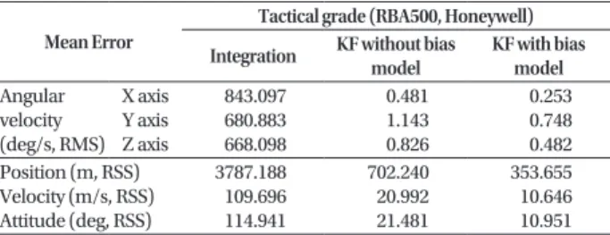
If the angular velocity is estimated using the extended Kalman filter in the gyro-free inertial navigation system, the effect of the accelerometer error and initial angular velocity error can be reduced. In this paper, in order to improve the navigation performance of the gyro-free inertial navigation system, an angular velocity estimation method is proposed based on an extended Kalman filter with an accelerometer random bias error model. In order to show the validity of the proposed estimation method, angular velocities and navigation outputs of a vehicle with 3 rev/s rotation rate are estimated. The results are compared with estimates by other methods such as the integration and an extended Kalman filter without an accelerometer random bias error model. The proposed method gives better estimation results than other methods.
Keywords: accelerometer bias, Extended Kalman Filter, gyro-free INS, MEMS, spinning vehicle
& Pachter 2005). Schuler et al. (1967) showed that rotational accelerations were measured from accelerometers arranged on a vehicle and angular velocities of the vehicle could be obtained by integrating measured rotational accelerations.
This accelerometers arrangement on the vehicle is called Gyro-Free IMU (GF-IMU) (Chen et al. 1994, Hanson &
Pachter 2005). Theoretically, the angular velocity vector in the three dimensional space can be obtained from outputs of six accelerometers (Schuler et al. 1967).
When angular velocities are estimated from six accelerometers, it is difficult to accurately determine the angular velocities if a direct impact, i.e., a high linear acceleration or a high angular acceleration is applied to the vehicle (Padgaonkar et al. 1975, Santiago 1992). To avoid this difficulty, a method using nine accelerometers was proposed (Padgaonkar et al. 1975). On the contrary, Chen et al. (1994) showed that angular velocities could be obtained by placing one accelerometer at the center of each face of a cube even though a direct impact is applied to the vehicle. In this arrangement, the sensing axis of each accelerometer is along the diagonal of respective cube face.
Received April 09, 2019 Revised May 07, 2019 Accepted May 27, 2019
†
Corresponding Author E-mail: [email protected]
Tel: +82-42-821-5670 Fax: +82-42-823-5436
Heyone Kim https://orcid.org/0000-0002-4291-3030
Junhak Lee https://orcid.org/0000-0002-4618-4728
Sang Heon Oh https://orcid.org/0000-0003-1357-0742
Dong-Hwan Hwang https://orcid.org/0000-0002-0933-5881
Sang Jeong Lee https://orcid.org/0000-0002-9400-5157
If angular velocities are estimated by integrating outputs of accelerometers, measurement errors of accelerometers are accumulated (Padgaonkar et al. 1975). In this case, navigation errors of the GF-INS increase more rapidly than those of SDINS, in which the angular velocity is measured using a gyroscope (Park et al.k 2005). Due to this characteristic, a method for reducing angular velocity estimation error is required in order to apply the GF-INS to long-term navigation.
Algrain & Saniie (1991) estimated the angular velocity using a static model between angular velocity and accelerometer output instead of integrating the accelerometer output.
They showed that effect of the Gaussian noise to the angular velocity estimate could be reduced by using a linear Gaussian estimator based on the linear model with the Gaussian noise.
Edwan et al. (2011) estimated angular velocities from accelerometer outputs using an extended Kalman filter with an accelerometer noise model. They showed that initial angular velocity error as well as the effect of the accelerometer noise could be reduced by considering dynamic characteristic between the angular velocity and accelerometer output. In addition to this, they showed through simulations that the random bias error of the accelerometer could be compensated by using an extended Kalman filter with only accelerometer noise model when a higher-grade accelerometer than the tactical-grade one is used.
Since the Micro-Electro Mechanical Systems (MEMS) accelerometer is smaller-sized and consumes lower power, it is suitable for very small-sized vehicles. Even though performance of the MEMS accelerometer has been improved and many research results on MEMS accelerometer based GF-INS can be found in literatures (Hanson 2005, Pachter et al. 2013, Cucci et al. 2016, Nilsson & Skog 2016, Chatterjee et al 2017), performance of the MEMS accelerometer still does not reach that of a conventional high-grade accelerometer (Hanson & Pachter 2005, Cucci et al. 2016). Therefore, in order for the GF-INS using MEMS accelerometer to give the same or similar performance of that using a high- grade accelerometer, the effect of the MEMS accelerometer error should be reduced more when the angular velocity is estimated (Cucci et al. 2016). As a method to this end, the angular velocity can be estimated from the accelerometer output using an extended Kalman filter with an accelerometer random bias error model.
In this paper, a GF-INS angular velocity estimation method is proposed based on an extended Kalman filter with an accelerometer random bias error model. The estimated angular velocity and navigation results are compared with those by other methods.
In the sequel, the angular velocity estimation algorithm using an extended Kalman filter is described. in Section 2. In Section 3, performance evaluation results of the proposed estimation method are presented. Finally, in Section 4, concluding remarks and further studies are given.
2. ANGULAR VELOCITY ESTIMATION USING EXTENDED KALMAN FILTER
2.1 Gyro-free INS Mechanization
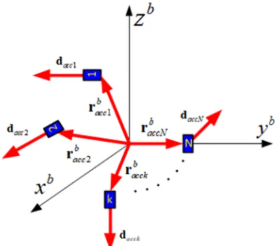
An arrangement of N accelerometers in a vehicle is shown in Fig. 1. When the vehicle moves, the acceleration of the point where the accelerometer is located is given in Eq. (1) (Schuler et al. 1967).
( )
b b b b b b b
accj
= + ω´
ib× r
accj+ ω
ib× ω r
ib×
accja a (1)
where a
b, ω
biband r
baccj(j =1, 2, …, N) are acceleration of the center of gravity of the vehicle represented in the body frame, the angular velocity of the body frame with respect to the inertial frame represented in the body frame and the vector from the center of gravity of the vehicle to the j-th accelerometer represented in the body frame, respectively.
Provided that the input axis orientation of the j-th accelerometer is d
Taccj, the acceleration measured by the j-th accelerometer is given in Eq. (2).
( )
( ( ))
b b b
accj accj accj accj ib
b b b b
accj ib ib accj accj
y = + ×
+ × × −
T T
T T
d r d ω´
d ω ω r d g
a
(2)
where g
bdenotes the gravitation, vector represented in the body frame. The measured acceleration vector by all accelerometers is given in Eq. (3).
Fig. 1. Accelerometer arrangement in the vehicle.
1 1 1 1 1 1 1
2 2 2 2 2 2
( ) ( ( ))
( ) (
( )
b b T T T b T b b b
acc acc acc acc acc acc ib ib acc
b b T T b T b T
acc acc acc acc ib acc acc
b
b b T T T b
accN accN accN accN accN
y y y
× × ×
×
= − +
×
r d d d g d ω ω r
r d d ω´ d g d
r d d d g
M M M a M 2
( ))
( ( ))
b b b
ib ib acc
T b b b
accN ib ib accN
× ×
× ×
ω ω r d ω ω r
M
(3)
Let the terms in Eq. (3) be represented as Eqs. (4-7).
1 2
b b b
acc acc accN
y y y
=
TY L (4)
1 1
2 2
( ( ))
( ( ))
( ( ))
T b b b
acc ib ib acc
T b b b
acc ib ib acc
T b b b
accN ib ib accN
× ×
× ×
=
× ×
d ω ω r d ω ω r N
d ω ω r
M (5)
1 1 1
2 2 2
( )
( )
( )
b T T
acc acc acc
b T T
acc acc acc
b T T
accN accN accN
×
×
=
×
r d d
r d d
B
r d d
M M (6)
1 2
T b T b T b
acc acc accN
=
TDg d g d g L d g (7) Let’s define A as Eq. (8).
3 1
3
( )
bib b
N N
× −
×
= =
ω´ T
A A B B B
A
a(8)
Angular velocity differential equation Eq. (9) and acceleration equation Eq. (10) can be obtained from Eq. (3).
3 3 3
b b b
ib ib ib
b b
ib
=
ω´ ×N+
ω´ ×N−
ω´ ×Nω A Y A Dg A N (9)
3 3 3
b b b
b b
N N N
× × ×
= A
aY A +
aDg A −
aN
a (10)
2.2 Four Accelerometer-triads on the Center of Gravity and Three Axes
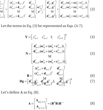
Consider the arrangement of accelerometers in Fig. 2.
Four accelerometer-triads are in the center of gravity and three axes (Hanson 2005, Edwan et al. 2011). In this case, the vectors from the center of gravity to the j-th accelerometer, r
baccj(j = 1, 2, …, 12), are given in Eqs. (11-14).
[ ]
1 2 3
0 0 0
b b b
acc
=
acc=
acc=
r r r (11)
[ ]
4 5 6
0 0
b b b
acc
=
acc=
acc=
r r r (12)
[ ]
7 8 9
0 0
b b b
acc
=
acc=
acc= l
r r r (13)
[ ]
10 11 12
0 0
b b b
acc
=
acc=
acc= l
r r r (14)
where l denotes the distance from the center of gravity to the accelerometer in the axis. Input axis orientations d
Taccj(j = 1, 2,
…, 12) are given in Eqs. (15-17).
[ ]
1 4 7 10
1 0 0
acc
=
acc=
acc=
acc=
T T T T
d d d d (15)
[ ]
2 5 8 11
0 1 0
acc
=
acc=
acc=
acc=
T T T T
d d d d (16)
[ ]
3 6 9 12
0 0 1
acc
=
acc=
acc=
acc=
T T T T
d d d d
(17)
Then, Eq. (18) is obtained from Eq. (8).
3 12
0 1 1 0 0 0 0 0 1 0 1 0
1 1 0 1 0 0 1 0 0 0 1 0 0
2 1 1 0 0 1 0 1 0 0 0 0 0
bib×
l
− −
= − −
− −
ω´
A (18)
Inserting Eq. (18) into Eq. (9), Eq. (19) is obtained (Algrain
& Saniie 1991).
1 2 3 4 5 6 7 8 9 10 11 12
( ) 0 1 1 0 0 0 0 0 1 0 1 0
( ) 1 1 0 1 0 0 1 0 0 0 1 0 0
( ) 2 1 1 0 0 1 0 1 0 0 0 0 0
bacc accb accb accb
b accb
ib x b
b acc
ib y b
b acc
ib z b
acc accb bacc accb bacc
y y y y y y
l y
y y y y y
−
= − −
− −
ω´ω´
ω´
(19)
where (ω
bib)
x, (ω
bib)
y, and (ω
bib)
zare x, y, and z axis component of ω
bib, respectively. Inserting Eqs. (11-17) into Eq. (10), Eqs. (20- 25) are obtained.
5 2 7 1
( ) ( ) 1 ( )
2
b b b b b b
ib x ib y
y
accy
accy
accy
acc= l − + −
ω ω (20)
( ) ( ) 1 (
6 3 10 1)
2
b b b b b b
ib x ib z
y
accy
accy
accy
acc= l − + −
ω ω (21)
9 3 11 2
( ) ( ) 1 ( )
2
b b b b b b
ib y ib z
y
accy
accy
accy
acc= l − + −
ω ω (22)
2
4 1 8 2 12 3
(( ) ) 1 ( )
2
b b b b b b b
ib x
y
accy
accy
accy
accy
accy
acc= l − − + − +
ω (23)
2
8 2 4 1 12 3
(( ) ) 1 ( )
2
b b b b b b b
ib y
y
accy
accy
accy
accy
accy
acc= l − − + − +
ω (24)
2
12 3 4 1 8 2
(( ) ) 1 ( )
2
b b b b b b b
ib z
y
accy
accy
accy
accy
accy
acc= l − − + − +
ω (25)
Fig. 2. 4 accelerometer-triads at the center of gravity and three axes.
2.2.1 Extended Kalman filter without accelerometer random bias error model
Let the state for the Kalman filter be given in Eq. (26).
1 2 3
[ x x x ] (
bib x) (
bib y) (
bib z)
=
T=
Tx ω ω ω (26)
If the probability distribution of the noise in the accelerometer output y
accj(j = 1, 2, …, 12) is white Gaussian, the process model Eq. (27) is obtained from Eq. (19).
1 2 3 4 5 6 7 8 9 10 11 12
( ) 0 1 1 0 0 0 0 0 1 0 1 0 ( ) 1 1 0 1 0 0 1 0 0 0 1 0 0 ( ) 2 1 1 0 0 1 0 1 0 0 0 0 0
b acc bacc bacc bacc
b bacc
ib x b
b acc
ib y b
b acc
ib z b
accb acc bacc accb bacc
y y y y y y
l y
y y y y y
−
= = − −
− −
ω´
x ω´
ω´
2 3 9 12
1 3 6 10
1 2 5 7
+1 2
acc acc acc acc
acc acc acc acc
acc acc acc acc
w w w w
w w w w
l w w w w
′ − ′ + ′ + ′
−′ + ′ − ′ + ′
′ ′ ′ ′
− + −
(27)
where w'
accj(j = 1, 2, …, 12) denotes white Gaussian noise of the j-th accelerometer. Relations between angular velocity and accelerometer output can be written in Eqs. (28-33) from Eqs.
(20-25).
5 2 7 1
5 2 7 1
( ) ( ) 1 ( )
2
1 ( ) 2
b b b b b b
ib x ib y
y
accy
accy
accy
accl
w w w w l
= − + −
′ ′ ′ ′
+ − + −
ω ω
(28)
6 3 10 1
6 3 10 1
( ) ( ) 1 ( )
2 1
( ) 2
b b b b b b
ib x ib z
y
accy
accy
accy
accl
w w w w l
= − + −
′ ′ ′ ′
+ − + −
ω ω
(29)
9 3 11 2
9 3 11 2
( ) ( ) 1 ( )
2 1
( ) 2
b b b b b b
ib y ib z
y
accy
accy
accy
accl
w w w w l
= − + −
′ ′ ′ ′
+ − + −
ω ω
(30)
2
4 1 8 2 12 3
4 1 8 2 12 3
(( ) ) 1 ( )
2
+ ( 1 )
2
b b b b b b b
ib x
y
accy
accy
accy
accy
accy
accl
w w w w w w l
= − − + − +
′ − ′ − ′ + ′ − ′ + ′ ω
(31)
2 8 2 4 1 12 3
8 2 4 1 12 3
(( ) ) 1 ( )
2
+ ( 1 )
2
b b b b b b b
ib y
y
accy
accy
accy
accy
accy
accl
w w w w w w l
= − − + − +
′ − ′ − ′ + ′ − ′ + ′ ω
(32)
2 12 3 4 1 8 2
12 3 4 1 8 2
(( ) ) 1 ( )
2 1
( )
2
b b b b b b b
ib z
y
accy
accy
accy
accy
accy
accl
w w w w w w l
= − − + − +
′ ′ ′ ′ ′ ′
+ − − + − +
ω
(33)
The measurement model Eq. (34) is obtained from Eqs.
(28-33).
2 2 2
1 2 1 3 2 3 1 2 3
( ) x x x x x x x x x
= + =
T+
z h x v v (34)
where v is given in Eq. (35).
5 2 7 1
6 3 10 1
9 3 11 2
4 1 8 2 12 3
8 2 4 1 12 3
12 3 4 1
acc acc acc acc
acc acc acc acc
acc acc acc acc
acc acc acc acc acc acc
acc acc acc acc acc acc
acc acc acc acc
w w w w
w w w w
w w w w
w w w w w w
w w w w w w
w w w w w
′ − ′ + ′ − ′
′ − ′ + ′ − ′
′ − ′ + ′ − ′
= ′ − ′ − ′ + ′ − ′ + ′
′ − ′ − ′ + ′ − ′ − ′
′ − ′ − ′ + ′ − ′ v
8 2
acc
w
acc
+ ′
(35)
The process model Eq. (27) can be discretized into Eq. (36) (Brown & Hwang 1997).
1
k+
=
k k+
k k+
kx Φ x Г u w (36)
where x
k, Φ
k, u
k, Γ
kand w
kare given in Eqs. (37-41), respectively.
, , ,
(
b) (
b) (
b)
k
=
ib x k ib y k ib z k
Tx ω ω ω (37)
1 0 0 0 1 0 0 0 1
k
=
Ф (38)
1, 2, 12,
b b b
k
= y
acc ky
acc ky
acc k
Tu L (39)
0 1 1 0 0 0 0 0 1 0 1 0
1 0 1 0 0 1 0 0 0 1 0 0
2 1 1 0 0 1 0 1 0 0 0 0 0
k
t
l
− −
∆
= − −
− −
Г (40)
2, 3, 9, 12,
1, 3, 6, 10,
1, 2, 5, 7,
acc k acc k acc k acc k
k acc k acc k acc k acc k
acc k acc k acc k acc k
w w w w
w w w w
w w w w
′ ′ ′ ′
− + +
′ ′ ′ ′
= − + − +
′ − ′ + ′ − ′
w (41)
The measurement z
kcan be written in Eq. (42) from Eq.
(34).
2 2 2
1, 2, 1, 3, 2, 3, 1, 2, 3,
1, 2, 3, 4, 5, 6,
( )
k k k k k k k k k k k k
k k k k k k
x x x x x x x x x
v v v v v v
= + =
+
T T
z h x v
(42) where v
kis given in Eq. (43).
5, 2, 7, 1,
6, 3, 10, 1,
9, 3, 11, 2,
4, 1, 8, 2, 12, 3,
8, 2, 4, 1,
acc k acc k acc k acc k
acc k acc k acc k acc k
acc k acc k acc k acc k
k acc k acc k acc k acc k acc k acc k
acc k acc k acc k acc k
w w w w
w w w w
w w w w
w w w w w w
w w w w
′ − ′ + ′ − ′
′ − ′ + ′ − ′
′ − ′ + ′ − ′
= ′ − ′ − ′ + ′ − ′ + ′
′ − ′ − ′ + ′ −
v
12, 3,
12, 3, 4, 1, 8, 2,
acc k acc k
acc k acc k acc k acc k acc k acc k