Influence of Gas Metal Arc Welding Parameters on the Bead Properties in Automatic Cladding

1. Introduction

Gas Metal Arc Welding (GMAW) is a process in which a continuous wire electrode and a shielding gas are fed through the nozzle of a welding gun. This proc- ess is widely found in the industry thanks to a high pro- ductivity and its potential to automation. It is primarily used for repairing worn out parts, applying corrosion re- sistant surfaces or metal joining in a large scale. This arc welding technique is used in particular for the re- building and improvement of the service life of rolls op- erating in metal to metal wear conditions.

The quality of the weld is critical and can be evaluated in various ways, in particular the characteristics of the weld bead geometry which plays an important role with regards to the mechanical properties of the weld

. The bead geometry is directly influenced by the welding process parameters

. To avoid weld bead defects and insure satisfactory mechanical properties, it is therefore necessary to carefully set-up the process parameters.

These parameters are welding current, arc voltage, weld- ing speed, torch angle, free wire length, nozzle-to-plate

distance, welding direction, position and the flow rate and composition of the shielding gas

.

It is often very costly and time consuming to optimize the welding process by experimental analysis. This is due to the effects and interactions of the numerous process parameters influencing the quality of the weld bead. This is why analytical approaches have been de- veloped using in particular designed experiments

.The Response Surface Methodology (RSM)

is one of those methods and has been widely used to study the weld bead geometry as a function of several process pa- rameters

.

In the present study, the RSM optimization technique is used to study the effects of welding parameters on the bead geometry of bead on plate welds deposited by GMAW on low-carbon steel. Four parameters are se- lected as input variables: welding speed (S), arc voltage (U), welding current (I) and shielding gas (SG). The re- sponses are: penetration (p), width (w), height (h), con- tact angle (θ), hardness (HR), dilution (D) and heat in- put (HI). A mathematical model is proposed for predict- ing the weld bead geometry and the optimal range for the parameters is given.

Influence of Gas Metal Arc Welding Parameters on the Bead Properties in Automatic Cladding

Mathieu TERNER* ^, †, Tsend-Ayush BAYARSAIKHAN**, Hyun-Uk HONG* and Je-Hyun LEE*

*Department of Materials Science and Engineering, Changwon National University, Changwon 51140, Korea

**Department of Mechatronics, School of Mechanical and Transportation, Mongolian University of Science and Technology, Ulaanbaatar 14191, Mongolia

†Corresponding author : [email protected]

(Received December 2, 2016 ; Revised December 23, 2016 ; Accepted January 3, 2017)

Abstract

Gas Metal Arc Welding is a widely used process in Industry due to its high productivity and potential to automation. The present study investigates the effects of the welding speed, arc voltage, welding current and shielding gas on the bead geometry for a low-carbon steel. The Response Surface Methodology (RSM) is used to choose an experimental design and perform test runs accordingly in order to produce mathematical models predicting the geometry, the hardness and the heat input of the bead as functions of the welding parameters.

The direct and interaction effects of the four welding parameters are represented graphically and allow to determine an optimum set of welding parameters.

Key Words : Gas metal arc welding, Welding parameters, Low carbon steels, Response surface methodology, Experimental design

ISSN 2466-2232

Online ISSN 2466-2100

2. Experimental section 2.1 Cladding process

The cladding experiments were carried out using a di- rect current inverter welding machine (JASIC-MIG250, 5 to 300 A output range) and a semiautomatic carriage (speed from 1 to 400 mm.min

). The cladding material was an AWS classification E-7012 solid wire (OK Autrod 13.12) with a diameter of 1.2 mm. The base metal were 20×20×100 mm plates of C-CH35ACR low carbon steel. The chemical compositions of the base material and the cladding wire are given in Table 1.

A critical parameter identified during trial runs was the wire feed rate (WF). This wire feed rate was propor- tional to the welding arc current (I) and followed a line- ar relationship. This relationship between the wire feed rate (WF) and the welding current (I) is given by Eq.

^{     } (1) The wire feed rate should be greater than a critical val- ue to avoid defects

. The wire feed rate and the weld- ing arc current accordingly were chosen to obtain sim- ilar welding bead profiles according to different weld- ing speed. The faster the welding speed, the fewer the melted wire deposited per unit length and therefore the smaller the bead geometry.

The shielding gas used for GMAW processes plays an important role. It can influence the quality and aspect of the welding joint, the welding speed and the actual costs of the process

. Boiko at al.

studied the effect of shielding gases on the MAG welding process. The different thermal conductivity of the shielding gases has

a considerable influence on the arc configuration and the bead geometry. In the present study, different shield- ing gases were used with between argon, CO

, O

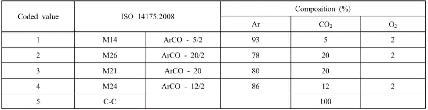
and mixture gases at a constant flow rate of 15 L/min. The standard names and composition of the gases are given in Table 2.

2.2 Experimental design

The experimental work in this study was carried out according to the Response Surface Methodology (RSM)

and was similar to previous similar studies

. This empirical method is commonly used for process in an industrial setting to optimize a response (here the bead geometry) influenced by several independent variables (here the process parameters). This method has been found to be valuable for the particular case of GMAW optimization

. As described for example by Bezerra et al.

, some stages in the application of RSM include:

(1) selection of independent variables of major effects on the system and delimitation of the experimental re- gion, (2) choice of the experimental design and ex- perimental runs according to the selected design matrix, (3) mathematical-statistical treatment of the obtained experimental data through the fit of a polynomial func- tion, (4) evaluation of the model’s fitness, (5) evalua- tion of the optimum values for each studied variables.

2.2.1 Process variables and response

The independent process variables identified as input parameters were adequately selected to carry out the ex- perimental work and develop the mathematical models.

The input variables were: welding speed (S), arc volt-

C Si Mn Cr Ni Cu Mo P S

Base metal: C-CH35ACR

mild steel 0.01-0.03 0.08-0.1 0.2-0.4 0.1 0.1 0.1 0.03 0.04

Welding wire: OK Autrod

13.12 0.1 0.5 1.1 0.5 0.5 0.2 0.03 0.03

Table 2 Standard name and chemical composition of the shielding gases

Coded value ISO 14175:2008 Composition (%)

Ar CO

O

1 M14 ArCO - 5/2 93 5 2

2 M26 ArCO - 20/2 78 20 2

3 M21 ArCO - 20 80 20

4 M24 ArCO - 12/2 86 12 2

5 C-C 100

Table 1 Chemical compositions of the base material and the welding wire

age (U), welding current (I) and shielding gas (SG). To describe the bead geometry, the responses or output pa- rameters were: penetration (p), width (w), height (h), contact angle (θ), hardness (HR), dilution (D) and heat input (HI).

2.2.2 Limits of the process variables

The lower and upper limit values of the process varia- bles were found by conducting trial runs and inspecting the bead for smooth appearance without any visible de- fects such as porosity, undercut, humping, etc. The low-

er limits were coded as -2 while the upper limits were coded as +2 according to the central composite rotat- able factorial design selected for this study. The inter- mediate levels (-1, 0 and +1) were determined by interpolation. The list of input variables and their values as per coded value are given in Table 3.

2.2.3 Design matrix

The design matrix chosen to conduct the experiment was a central composite rotatable design consisting in 32 coded conditions. The design matrix is constituted of

Input variable Unit Notation Level

-2 -1 0 +1 +2

Welding speed cm/min S 30 50 70 90 110

Arc voltage V U 19 21 23 25 27

Welding current A I 180 210 240 270 300

Shielding gas % SG 1 2 3 4 5

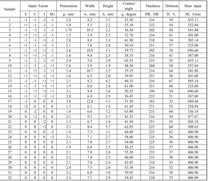
Table 4 Design matrix and measured or calculated values of the responses Sample Input Factor Penetration Width Height Contact

angle Hardness Dilution Heat input

S U I SG p, mm w, mm h, mm q, degree HR, HB D, % HI, J/mm

1 -1 -1 -1 -1 2.6 8.2 3.1 53.50 216 54 455.11

2 +1 -1 -1 -1 1.9 5.5 2.2 55.10 232 54 252.84

3 -1 +1 -1 -1 1.75 10.3 2.2 36.30 202 56 541.80

4 +1 +1 -1 -1 1.5 5.9 2.3 52.70 216 61 301.00

5 -1 -1 +1 -1 2.8 8.8 3.3 61.90 210 54 585.14

6 +1 -1 +1 -1 2.1 7.6 2.8 50.10 251 57 325.08

7 -1 +1 +1 -1 2.6 10.9 3.1 39.75 202 54 696.60

8 +1 +1 +1 -1 1.6 9.4 2.5 38.35 216 61 387.00

9 -1 -1 -1 +1 2.4 5.8 2.9 65.35 233 55 455.11

10 +1 -1 -1 +1 1.6 5.9 1.9 48.50 260 54 252.84

11 -1 +1 -1 +1 1.4 10.7 2.5 35.35 216 64 541.80

12 +1 +1 -1 +1 1.6 6.5 2.0 39.95 251 56 301.00

13 -1 -1 +1 +1 2.1 9.2 4.2 60.35 216 67 585.14

14 +1 -1 +1 +1 1.9 6.0 2.8 61.00 251 60 325.08

15 -1 +1 +1 +1 3.1 9.4 3.6 50.25 196 54 696.60

16 +1 +1 +1 +1 2.8 6.9 2.9 56.45 233 51 387.00

17 -2 0 0 0 3.0 12.8 3.3 51.50 183 52 949.44

18 +2 0 0 0 1.3 6.1 1.6 41.45 271 55 258.94

19 0 -2 0 0 1.8 6.6 3.2 63.90 233 64 336.14

20 0 +2 0 0 2.1 9.3 2.5 41.55 216 54 477.67

21 0 0 -2 0 1.3 6.7 1.6 41.50 251 55 305.18

22 0 0 +2 0 2.1 8.4 3.7 62.95 225 64 508.63

23 0 0 0 -2 1.9 7.3 3.1 64.40 225 62 406.90

24 0 0 0 +2 2.1 7.1 2.7 58.60 225 56 406.90

25 0 0 0 0 2.1 7.0 2.7 54.00 225 56 406.90

26 0 0 0 0 1.9 6.8 2.5 50.25 233 57 406.90

27 0 0 0 0 2.1 7.0 2.8 55.20 233 57 406.90

28 0 0 0 0 2.5 7.4 2.5 46.60 233 50 406.90

29 0 0 0 0 2.1 7.8 2.4 42.45 216 53 406.90

30 0 0 0 0 2.4 7.5 2.6 53.30 216 52 406.90

31 0 0 0 0 2.2 6.8 3.0 59.95 216 58 406.90

32 0 0 0 0 2.4 7.1 2.9 54.45 210 55 406.90

Table 3 Input variables selected for the RSM and their levels

a full replication of 2

(16) factorial design, 8 star points (one variable at its highest level +2 or lowest level -2 with all the other variables at the intermediate level 0) and 8 center points (all variables at the intermediate lev- el 0). In this way, the 32 experimental runs allowed the estimation of linear, quadratic and linear-linear inter- active effects of the welding parameters on the bead geometry. The design matrix is given in Table 4.

2.2.4 Experimental work according to the design ma- trix and record of the responses

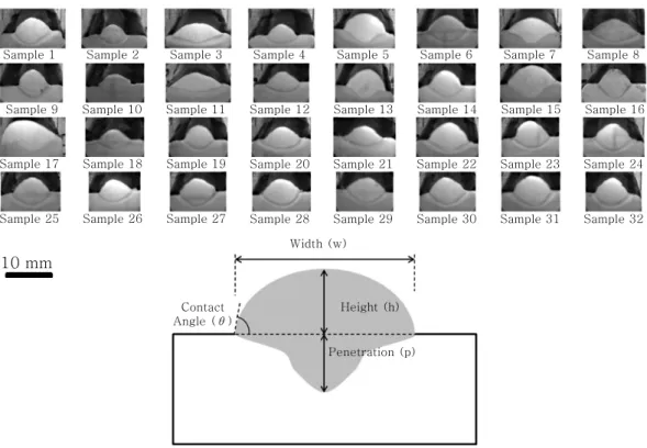
The 32 experimental runs as described in the design matrix (Table 4) were realized for the four welding pa- rameters selected as the input parameters. The bead on plate welds were subsequently cut and the cross section of the beads were polished and observed by optical microscopy. Figure 1 shows the photographs of the 32 specimens where the bead geometry could be studied.

The profiles of the beads for the different sets of param- eters were traced using an image analysis software so that the bead geometry could be measured accurately.

Figure 1 also shows a schematic drawing of a bead on plate profile. For each single experimental run, the bead geometry was defined by measuring several out param- eters: the width (w), the height (h), the penetration (p) and the contact angle (θ).

The percentage of dilution, hereafter referred to as di- lution, was calculated for each weld. The dilution is de- fined in Eq. (2) as the ratio between the penetration p to

the total height of the bead profile p+h in Fig. 3. The basic difference between welding and cladding is this percentage of dilution which should be as low as possi- ble in cladding. The lower the dilution the closer is the composition of the bead to that of the filler material.

     ×  (2)

Where p is the penetration (mm) and h is the height (mm) as described in Fig. 1.

The Heat input (HI) was also calculated for each run.

Heat input is a relative measure of the energy trans- ferred per unit length of welding bead. It is an important characteristic because, similarly to preheat and in- ter-pass temperatures, it influences the cooling rate which may affect the mechanical properties and metal- lurgical structure of the weld and the HAZ

. The heat input is typically calculated as the ratio of the power to the velocity of the heat source, as described in Eq. (3):

^{  }

  × 

 ×  × 

(3) Where 

=0.86 is the heat transfer efficiency

, I is the welding current (A), U is the arc voltage (V) and S is the welding speed (cm/min).

Finally, the Brinell hardness was measured (Dia testor 2Rc, Wolpert). The results of the measurements and cal- culations are given in Table 4 for the 32 samples, each one defined by a set of parameters as described previously.

Sample 1 Sample 2 Sample 3 Sample 4 Sample 5 Sample 6 Sample 7 Sample 8

Sample 9 Sample 10 Sample 11 Sample 12 Sample 13 Sample 14 Sample 15 Sample 16

Sample 17 Sample 18 Sample 19 Sample 20 Sample 21 Sample 22 Sample 23 Sample 24

Sample 25 Sample 26 Sample 27 Sample 28 Sample 29 Sample 30 Sample 31 Sample 32

10 mm

Width (w)

Contact Angle (θ)

Height (h)

Penetration (p)

Fig. 1 Photographs of the bead profile in cross section for the 32 samples and schematic representation of the weld bead

geometry

2.2.5 Development of the mathematical models The response function representing any of the re- sponses defined earlier can be expressed as a function of the input parameters, as in the following Eq. (4):

           (4)

Where Y is the response and S, U, I and SG are the welding speed, the arc voltage (U), the welding current (I) and the shielding gas (SG) respectively. A second- degree polynomial equation, a model commonly used in RSM

, was selected for the four input variables to represent the response and is given in Eq. (5):

  β

 

  



β



 

  



β



 

  



β





 ε (5)

Where Y is the response,

is the constant term,

rep- resents the coefficient of the linear parameters,

rep- resents the coefficients of the quadratic parameter,

represents the coefficients of the interaction parameters,

_

(or

) represents the input variables (S, U, I and SG) and ε is the residual associated to the experiments. The values of the coefficients in Eq. (5) were calculated by fitting the functions to the data using a statistical soft- ware (STATISTICA, Excel S-PLUS 8.0). A computer program was also developed to calculate the value of these coefficients for different responses (Table 5).

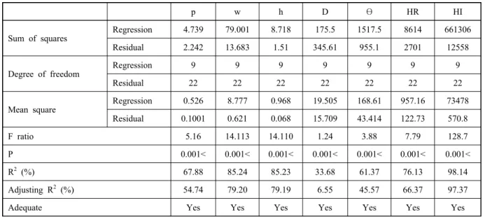
The adequacy of the models was tested using the anal- ysis of variance (ANOVA). According to this technique, if the calculated values of the F ratio of the developed model do not exceed the standard tabulated values for the desired level of confidence (95%) and the calculated values of the R ratio of the developed model exceed the standard values for the desired level of confidence (95%),

then the model can be considered adequate within the confidence limit. The results in Table 5 show that all the models are adequate.

The coefficients obtained for each response were test- ed for significance. The value of the coefficients gives an idea as to what extent the control variables affect the responses quantitatively. The less significant coefficients can be eliminated for the response which they are asso- ciated to. To achieve this, Student’s t-test is commonly used. According to this test, when the calculated values of t corresponding to a coefficient exceed the standard tabulated values for the desired level of probability (95%), the coefficient becomes significant. Accordingly, the models were developed considering only significant coefficients.

The final mathematical models as determined by the above analysis are given Eqs (6)-(12) for the responses considered:

P(penetration,mm)=11.7317-0.0409S-0.561U+0.0167I -0.0093U

+0.0016SU+0.0036UI (6) h(height,mm)=12.16-0.0533S-0.8805U+0.0195I

+0.012U^2+0.0033SU-0.001SI (7) w(width,mm)=7.7397-0.131S-0.2998U+0.0277I

+0.0014S

+0.0445U

-0.0088SU

+0.0031UI (8)

D(dilution,%)=39.0122-0.1335S-1.8733U+0.3622I -0.0012S

+0.2177U

+0.0011I

+0.0082SU-0.0379UI (9)

θ(contact angle,degree)=147.43-0.9097S-6.0056U +0.2719I-0.005S^2-0.1143U

p w h D θ HR HI

Sum of squares Regression 4.739 79.001 8.718 175.5 1517.5 8614 661306

Residual 2.242 13.683 1.51 345.61 955.1 2701 12558

Degree of freedom Regression 9 9 9 9 9 9 9

Residual 22 22 22 22 22 22 22

Mean square Regression 0.526 8.777 0.968 19.505 168.61 957.16 73478

Residual 0.1001 0.621 0.068 15.709 43.414 122.73 570.8

F ratio 5.16 14.113 14.110 1.24 3.88 7.79 128.7

P 0.001< 0.001< 0.001< 0.001< 0.001< 0.001< 0.001<

R

(%) 67.88 85.24 85.23 33.68 61.37 76.13 98.14

Adjusting R

(%) 54.74 79.20 79.19 6.55 45.57 66.37 97.37

Adequate Yes Yes Yes Yes Yes Yes Yes

Table 5 Calculation of variance for testing the models

+0.0816SU-0.0013SI

+0.01UI (10)

HR(hardness,HB)=342.67+0.46S+6.534U-1.5179I -0.0012S

-0.0385U

+0.0036I

-0.0297SU+0.0036SI-0.026UI (11) HI(heat input,J/mm)= -221.14-10.992S+42.0095U+2.8751I

+0.1182S

-0.5059U

-0.0021I

-0.2752SU-0.264SI+0.0803UI (12) In the following Results and Discussion section, the direct and interaction effects of the selected welding pa- rameters on the bead geometry, dilution, hardness and heat input are presented graphically. Based on these models and considering legitimate constraints on the parameters and responses, the optimal set of welding parameters could be determined.

3. Results and Discussion

The mathematical models given in the previous sec- tion can be used to predict the weld bead geometry, di- lution, hardness and heat input considering a given set of parameters. More importantly, these models can be used to select the proper values of the welding parame- ters considered in order to maximize the quality of the weld. Based on the models, the main and interaction ef- fects of the process parameters were computed and plotted.

3.1 Direct effects of the welding parameters on the weld bead

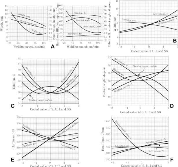
The direct effect of the welding speed S on the bead geometry (p, h, w and θ), the dilution (D), the hardness (HR) and the heat input (HI) is given graphically in Fig.

2A. From this figure, while the hardness increases quasi linearly with the welding speed, the height (h), pene- tration (p) and width (w) decrease significantly. This is not surprising since when the welding speed increases, the volume of metal deposited per unit length decreases.

The contact angle (θ) initially increases by more than 5°

when the welding speed increases from 30 to about 65 cm/min and then decreases down to its lowest value at S = 110 cm/min. The effect of the welding speed on dilu- tion (D) is discussed later (Fig. 2C). The heat input (HI) quickly decreases when the welding speed increases un- til it reaches a minimum value slightly under 300 J/mm for S ≈ 100 cm/min. In practice, it is of great industrial interest to maximize welding speeds in order to increase the productivity of a particular welding operation

.

The direct effects of the process variables on the bead width (w) are shown in Fig. 2B. The width of the weld- ing bead is important in cladding with wider bead being preferred. From Fig. 2B, the bead width increases sig- nificantly when both the arc voltage (U) and the weld- ing current (I) increase. It is also noted that the bead width slightly decreases when the amount of CO

in the shielding gas increases. From Fig. 2A, it was seen that the width decreases when the welding speed increases, as discussed earlier.

The direct effects of the process variables on the dilu- tion (D) are shown in Fig. 2C. The general trend in Fig.

2C is that the dilution decreases initially when the val- ues of the arc voltage (U), the welding current (I) and the shielding gas (SG) get close to their coded value 0 (refer to Table 3) and increases after that. Inversely, when the welding speed initially increases up to its coded value 0, the dilution also increases and then decreases af- ter that.

The direct effects of the process variables on the con- tact angle (θ) are shown in Fig. 2D. It can be seen that the contact angle of the bead on the plate is very sensi- tive to the welding parameters. When the arc voltage (U) increases, the contact angle quickly decreases. However, when the welding current (I) increases, the contact an- gle quickly increases. When the welding speed (S) ini- tially increases up to its coded value 0 (70 cm/min), the contact angle also increases. It decreases however when the welding speed is further increased. The nature of the shielding gas also has a significant effect on the contact angle, its lowest value being for SG having the coded value of 0 (SG = M21)

The direct effects of the process variables on the bead hardness (HR) are shown in Fig. 2E. As previously men- tioned, it can be seen in Fig. 2E that the welding speed has a great influence on the hardness of the bead. The hardness of the bead quickly increases apparently line- arly when the welding speed (S) increases. The nature of the shielding gas (SG) also has a significant impact on the hardness of the bead. It is also seen in Fig. 2E that the hardness quickly decreases when the arc volt- age (U) increases. Finally, the hardness of the bead de- creases when the welding current increases up to about 255 A and slightly increases after that.

The direct effects of the process variables on the heat

input (HI) are shown in Fig. 2F. From this figure, it ap-

pears that the nature of the shielding gas has very little

influence on the heat input. Also, the input similarly in-

creases when the welding current (I) and arc voltage

(U) increase. Finally, the heat input decreases when the

welding speed (S) increases. This is obviously consistent

with the measure of the heat input as given in Eq. (3).

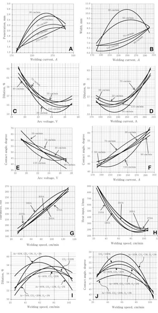
3.2 Interaction effects of the welding parameters on the weld bead

The interaction effects of the welding current (I) and the welding speed (S) on penetration (p) is shown in Fig. 3A. It can be seen that penetration increases ini- tially when the welding current increases, and the lower the welding speed the higher the increase. The pene- tration start decreasing when a certain value of welding current is attained and the lower the welding speed the lower this value. Interestingly, penetration is rather sim- ilar at low and high welding current regardless of the welding speed. However, and as could be expected, penetration tends to increase when the welding speed decreases at intermediate levels of welding current.

The interaction effects of the welding current (I) and the welding speed (S) on the bead width (w) is shown in Fig. 3B. At high welding speed, the bead width significantly increases when increasing the welding current. At lower welding speed, the width initially increases quickly when

the welding current increases and then decreases.

The interaction effects of the arc voltage (U) and the welding speed (S) on the dilution (D) is shown in Fig.

3C. From this figure, it is evident that at all welding speed, the dilution quickly decreases when the arc volt- age increases. At higher voltage, the dilution slightly increases.

The interaction effects of the welding current (I) and the welding speed (S) on the dilution (D) is shown in Fig. 3D. It is shown that the dilution slightly decreases initially and then quickly increases when the welding current increases.

The interaction effects of the arc voltage (U) and the welding speed (S) on the contact angle (θ) is shown in Fig. 3E. It can be seen that the contact angle decreases when the arc voltage increases. The effect is even more pro- nounced when the welding speed is 50 cm/min.

The interaction effects of the welding current (I) and the welding speed (S) on the contact angle (θ) is shown in Fig. 3F. It can be seen that the contact angle increases

14 13 12 11 10 9 8 7 6 5

Width, mm

Welding speed, cm/min

25 45 65 85 105

4.5 4.0 3.5 3.0 2.5 2.0 1.5 1.0 0.5 0.0 Height, mm

Penetration, mm Width, mm

Penetration, height, mm

1000 900 800 700 600 500 400 300 200 100

Welding speed, cm/min

25 45 65 85 105

70 65 60 55 45 40 35 30 25 20

HardnessHB, heat input, J/mm

Dilution, %

Dilution %, contact angle, degree

Conract angle

Heat input, J/mm

Hardness, HB

11

10

9

8

7

6

5

Width, mm

Coded value of U, I and SG

-2 -1 0 1 2

Arc voltage, V

Shielding gas

Welding current, A

B

62

61

60

59

58

57

56

-2 -1 0 1 2

Arc v oltag

e, V

Shielding gas Welding current, A

Coded value of S, U, I and SG

Dilution, %

55

54

65

60

55

50

45

40

-2 -1 0 1 2

Arc vo ltage, V Shielding gas

Welding current, A

Coded value of S, U, I and SG

Contact angle, degree

35

Welding speed, cm/min

260

250

240

230

220

210

-2 -1 0 1 2

Arc voltage, V Shielding gas

Weldin g curre

nt, A

Coded value of S, U, I and SG

Hardness,HB

200

190

Welding speed, cm/min 850

750

650

550

450

-2 -1 0 1 2

Arc voltage, V Shielding gas

Welding current, A

Coded value of S, U, I and SG

Heat Input, J/mm

350

250 Weld

ing s peed

, cm /min

A

Welding speed, cm/min

C D

E F

Fig. 2 Direct effects of the welding parameters on the weld bead

3.0

2.8

2.6

2.4

2.2

2.0

Welding current, A

Penetration, mm

1.8

1.6

1.4

1.2

170 220 270 320

11.0 10.5 10.0 9.5 9.0

Welding current, A

Width, mm

8.5 8.0 7.5

7.0

6.0

170 270 290

6.5

190 210 230 250 310

30 cm/min

50 cm/min

70 cm/min

110 cm/min

90 cm/min

30 cm/min 50 cm/min

70 cm/min

110 cm/min 90 cm/min

61

59

57

55

53

Dilution, %

Welding current, A 63

170 190 210 230 250 270 290 310

30 cm/min 50 cm/min

70 cm/min

110 cm/min

90 cm/min

Contact angle, degree

18 20 22 24 26 28

Arc voltage, V

60

55

50

45

40

30 cm/min

50 cm/min 70 cm/min

110 cm/min

90 cm/min 30 cm/min

50 cm/min

70cm/min

90cm/min 110cm/min

110 cm/min 30 cm/min

50 cm/min 70 cm

/min 90 cm/min

18 20 22 24 26 28

Arc voltage, V 61

59

57

55

53

Dilution, %

63

70

65

60

55

50

45

40

35

Welding current, A

170 190 210 230 250 270 290 310

40

Contact angle, degree

A B

C D

F E

Ar-86%, CO₂-12%, O₂-2%

CO₂-100%

Ar-93%, CO₂-5%, O₂-2%

Ar-80%, CO₂-20%

60

58

56

54

52

50

25 45 65 85 105

800

700

600

400

300 900

500

200

45

25 65 85 105 125

Welding speed, cm/min 210A

180A

300A 240A

270A

Ar-78%, CO₂-20%, O₂-2%

270A 180A

300A

210A 270

260

250

240

230

220

210

200

190

180

240A

Heat input, J/mm

40

20 60 80 100 120 120

Welding speed, cm/min

Hardness,HB

200

Dilution, % Contact angle, degree

Welding speed, cm/min Welding speed, cm/min

CO₂-100% Ar-93%, CO₂-5%, O₂-2%

Ar-80%, CO₂-20%

Ar-86%, CO₂-12%, O₂-2%

Ar-78%, CO₂-20%, O₂-2%

25 45 65 85 105

59

57

55

53

51

49

47

45

43

41

G H

I J

Fig. 3 Interaction effects of the welding parameters on the weld bead

when the welding current increases. The contact angle is overall the lowest at high welding speed of 110 cm/min and the highest at welding speed of 70 cm/min The interaction effect of the welding current (I) and the welding speed (S) on the hardness (HR) is shown in Fig. 3G. From this figure, it is evident that the hardness significantly increases with welding speed (as in Fig.

2E). The welding current only has a slight effect on the hardness when varying welding speed. The hardness is slightly higher when the welding current is lower.

The interaction effect of the welding current (I) and the welding speed (S) on the heat input (HI) is shown in Fig. 3H. The heat input quickly decreases when the weld- ing speed decreases which is consistent to Fig. 2F. The welding current only has a little effect and obviously, the lower heat input is obtained for low current.

Finally, the interaction effect of the shielding gas (SG) and the welding speed (S) on both the dilution (D) and the contact angle (θ) are shown in Fig. 3I and Fig. 3J respectively. It appears from Fig. 3I that at low and me- dium welding speed, the dilution is significantly higher when the content of CO

is lower in the mixture. The na- ture of the shielding gases also shows great influence on the contact angle when varying the welding speed (Fig.

3J), in particular when the welding speed is between 45 and 85 cm/min.

In order to appropriately select the optimal set of welding parameters, a certain number of key conditions should be determined. First, the welding speed should be as high as possible in order to maximize the productivity.

However, when the welding speed was higher than the upper value 110 cm/min, the arc was unstable and de- fects appeared

. The dilution should be as low as possible.

As it was mentioned before, high dilution is suitable for weld joint while low dilution is preferred in cladding or surfacing. When the dilution is low the final composi- tion of the deposited material is closer to that of the ac- tual filler material. Ideally, the dilution in such cladding process should be lower than 50 %. In the present study, considering the results presented in Figs. 2C, 3C, 3D, and 3I, the upper limit for the dilution (D) should be no more than 57 %. The contact angle (θ) also has a sig- nificant influence on the mechanical properties of the weld. It is usually sought a high contact angle of about 70° to 90°, where the bead profile looks like half a disc.

To insure satisfying conditions in the present study and considering Figs. 2A, 2D, 3E, 3F and 3J, the contact an- gle should be higher than 45°. At last, the heat input (HI) influences the cooling rate and in turn the microstructure of the bead. In the conditions of the present study, con- sidering Figs. 2A, 2F and 3H, the heat input should be

close to 400 J/mm or more. Based on these consid- eration and the results given graphically according to the mathematical model built in section 2.2.5, the fol- lowing conclusions can be drawn regarding the welding parameters considered in this study: the welding speed should be S ≈ 60 cm/min, the welding current should be I ≈ 200-250 A, the arc voltage should be U ≈ 20-25 V and the shielding gas should be SG = M21 (80%

Ar-20% CO

) for GMAW cladding on low-carbon steel.

4. Conclusion

The present study investigates the effects of four weld- ing parameters (welding speed (S), arc voltage (U), welding current (I) and shielding gas (SG)) on the bead geometry of bead on plate for a low-carbon steel. Based on the Response Surface Methodology (RSM), mathe- matical models were developed to predict the geometry, the hardness and the heat input of the bead as functions of the welding parameters. These models can easily be used in automatic cladding for obtaining weld bead of desired quality. The direct and interaction effects of the four welding parameters allowed determining an opti- mum set of parameters. In the conditions of the present study, the welding speed should be S ≈ 60 cm/min, the welding current should be I ≈ 200-250 A, the arc volt- age should be U ≈ 20-25 V and the shielding gas should be SG = M21 (80% Ar-20% CO

).

Acknowledgements

This research was financially supported by the National Research Foundation of Korea (NRF) funded by the Korean government (MSIP) (No. 2011-0030058). This research was supported by Changwon National University in 2016.

References

1. D.S. Correia, C.V. Goncalves, S.S. da Cunha Jr., V.A.

Ferraresi, Comparison between genetic algorithms and response surface methodology in GMAW welding opti- mization, J. Mater. Process Tech. 160 (2005), 70-76 2. P.K. Palani, N. Murugan, Optimization of weld bead ge-

ometry for stainless steel claddings deposited by FCAW, J. Mater. Process Tech. 190 (2007), 291-299

3. C. Doumanidis, Y.M. Kwak, Multivariable adaptive con- trol of the bead profile geometry in gas metal arc weld- ing with thermal scanning, Int. J. Pres. Ves. Pip. 79 (2002), 251-262

4. T.C. Nguyen, D.C. Weckman, D.A. Johnson, H.W. Kerr, High speed fusion weld bead defects, Sci. Technol.

Weld. Joi. 11 (6) (2006), 618-633

5. T.C. Nguyen, D.C. Weckman, D.A. Johnson, The dis- continuous weld bead defect in high-speed gas metal arc welds, Weld. J. 86 (2007), 360-3725

6. E. Karadeniz, U. Ozsarac, C. Yildiz, The effect of proc- ess parameters on penetration in gas metal arc welding processes, Mater. Des. 28 (2007), 649-656

7. R. Choteborsky, M. Navratilova, P. Hrabe, Effects of MIG process parameters on the geometry and dilution of the bead in the automatic surfacing, Res. Agr. Eng. 57 (2) (2011), 56-62

8. P. Sreeraj, T. Kannan, S. Maji, Optimization of weld bead geometry for stainless steel cladding deposited by GMAW, Am. J. Eng. Res. 02 (05) (2013), 178-187

9. P. Sreeraj, T. Kannan, S. Maji, Prediction and optimization of weld bead geometry in gas metal arc welding process using RSM and fmincon, J. Mech. Eng. Res. 5 (8) (2013), 154-165

10. P. Sreeraj, T. Kannan, S. Maji, Prediction and optimization of stainless steel cladding deposited by GMAW process using response surface methodology, ANN and PSO, Int. J. Eng. Sci. 3 (5) (2013), 30-41

11. P. Sreeraj, T. Kannan, S. Maji, Optimization of GMAW process parameters using particle swarm optimization, ISRN Metall. 2013, 1-10

12. I.S. Kim, K.J. Son, Y.S. Yang, P.K.D.V. Yaragada, Sensitivity analysis for process parameters in GMA welding proc- esses using a factorial design method, Int. J. Mach.

Tool. Manu. 43 (2003), 763-769

13. I. Boiko, D. Avisans, Study of shielding gases for MAG welding, Mater. Phys. Mech. 16 (2013), 126-134 14. R.H. Myers, D.C. Montgomery, C.M. Anderson-Cook,

Response Surface Methodology - Process and product optimization using designed experiments, John Wiley

& Sons, Hoboken, New Jersey (2009), 705

15. M.A. Bezerra, R.E. Santelli, E.P. Oliveira, L.S. Villar, L.A.

Escaleira, Response surface methodology (RSM) as a tool for optimization in analytical chemistry, Talanta 76 (2008), 965-977

16. O. Popovic, R. Prokic-Cvetkovic, M. Burzic, Z. Milutinovic, The effect of heat input on the weld metal toughness of surface welded joint, 14

Int. Res./Exp. Conf., TMT 2010 (11-18 September, 2010), 61-64

17. C.L. Jennery, A. O’Brien, Welding Handbook - Welding Science and Technology, American Welding Society, Miami, Florida (2001), 985 (54)

18. A.I. Khuri, S. Mukhopadhyay, Response surface meth-

odology, WIREs Comp. Stat. 2 (2012), 128-149