1. Introduction
Radars are wireless detection devices that transmit electromagnetic waves to a target and interprets reflected
*Corresponding author, E-mail: [email protected] Copyright ⓒ The Korea Institute of Military Science and Technology
waves from the target.
As RADAR stands for RAdio Detection And Ranging[4], radar systems identify distances, directions, and altitudes to a target.
Model and Simulation (M&S) is a technology to reproduce real world objects into simulation objects in computer systems, and it observes them what happen Research Paper 체계공학 부문
유도무기 임무 분석을 위한 레이더 성능 모델
김진규*,1) ․ 우상효1)
1)국방과학연구소 제1기술연구본부
A Radar Performance Model for Mission Analyses of Missile Models
Jingyu Kim*,1) ․ S. H. Arman Woo1)
1)The 1st Research and Development Institute, Agency for Defense Development, Korea
(Received 20 January 2017 / Revised 6 November 2017 / Accepted 24 November 2017)
ABSTRACT
In M&S, radar model is a software module to identify position data of simulation objects. In this paper, we propose a radar performance model for simulations of air defenses. The previous radar simulations are complicated and difficult to model and implement since radar systems in real world themselves require a lot of considerations and computation time. Moreover, the previous radar simulations completely depended on radar equations in academic fields; therefore, there are differences between data from radar equations and data from real world in mission level analyses. In order to solve these problems, we firstly define functionality of radar systems for air defense. Then, we design and implement the radar performance model that is a simple model and deals with being independent from the radar equations in engineering levels of M&S. With our radar performance model, we focus on analyses of missions in our missile model and being operated in measured data in real world in order to make sure of reliability of our mission analysis as much as it is possible. In this paper, we have conducted case studies, and we identified the practicality of our radar performance model.
Key Words : Radar Model, Performance Model, Missile Model, Mission Analysis, M&S, Guided Missile Simulation
among them in certain time and space. In M&S, four essential elements should be defined: time, events, actors, and space[2]. In defense domain, mission planning results of a missile model should be evaluated, and M&S is an only way to analyze the results of mission planning except for Live Fire Testing (LFT). For the mission analyses of our missile models through M&S, we should model and define the four essential elements for air defense systems. In modeling an air defense, reliabilities of radar systems and defensive weapon systems are one of significant factors.
In defense domain, M&S is classified into engineering, engagement, and mission level[9]. In this paper, we focus on radar simulations for air defenses in mission level. In the previous works, radar simulations are complicated and difficult to model and implement in computer systems because there are a lot of considerations and computing powers in real world. Moreover, the previous radar simulations completely depended on radar equations in academic fields, and we cannot ignore differences between data from radar equations and data from real world in mission level analyses.
In order to deal with these problems, we firstly define functionality of radar systems for air defenses to design the radar performance model. Then, we implement the radar model as simple as possible, and we make the simple radar model to comply with the model-based design[8] and deal with being independent from the radar equations.
With our radar performance model, we aim to carry out analyses of missions in our missile model and being operated in measured data in real world in order to make sure of reliability of our mission analysis as much as possible. Finally, in this paper, we attempt to prove practicality of the radar performance model with a case study. (This paper is an extended version of our previous research[1]).
The remainder of this paper is organized as follows:
Section 2 provides the research motivation in our experiences; Section 3 presents the design of our radar performance model for air defense; In Section 4, we conduct case studies; At the conclusion, Section 5 summarizes the contributions of this paper.
2. Research Motivation
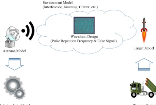
In M&S, air defense weapon systems consist of rule set model, Surface-to-Air Missile (SAM) model and radar model. The rule set model indicates operational logics such as assigning target-missile of priority and scheduling fire-time of SAM objects[11]. The SAM model is a set of equations of motion of missile objects. The radar model is a detection mechanism for flying objects that constitute threats to assets. Fig. 1 shows end-to-end radar processes in pulse radar applications.
Fig. 1. Traditional radar system
Radar systems transmit wave signals to a certain direction, and the signals transform echo signals by hitting a target object. Finally, radar systems obtain the echo signals and interpret them for position and speed data of the target. In other words, they obtain positions of targets by calculating delays of the echo signals and speed of targets through doppler shift[4].
In views of functionality of radar systems, these systems require waveform designs and antenna models that transmit/receive the designed waveform into/from wireless environments. In addition, the antenna models should be considered with its size and geometry in their performances.
In M&S, radar systems further require environment models that distort waveform and echo signals by interference, jamming, cluster, etc. Furthermore, these systems require target models for simulating generations of echo signals. Finally, radar systems interpret the echo
signals using independently designed data analysis models.
These complicated radar systems are difficult to model and implement in views of reproducing them in computer systems. These models require a lot of processing time in our experiences since longer flying time of our missile models and their precisely sampled period produce considerable input data to each model in a traditional radar system.
In M&S, these radar systems are implemented with a set of radar equations; however, there are differences between data from radar equations and measured data in real world. These differences are critical to results of mission analysis of our missile models in reliability.
Therefore, in this paper, we transform these complex radar systems into a simple model for analyzing mission planning results of our missile models based on time and spatial domains. In the following section, we will discuss the design solutions of our simple radar model.
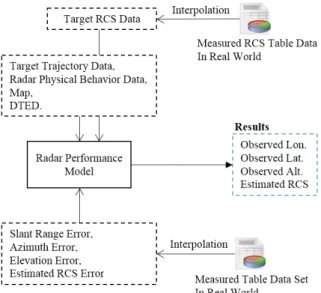
Fig. 2 illustrates the concept of our radar model.
Fig. 2. The concept of the radar model
Our radar performance model is designed only for mission analyses of our missile models in mission simulation level. Target trajectory (from our missile models), radar physical behavior, map, and Digital Terrain Elevation Data (DTED) are inputted into the radar model. In addition, table data such as real Radar
Cross Section (RCS) data, slant range error, azimuth error, elevation error, and estimated RCS error are inputted into the radar model, and the model interpolates these data for computing observations. These table data were actually measured in real world; therefore, we could be escaped from the engineering levels of radar equations. Finally, the radar performance model produces observed longitude, latitude, altitude, and estimated RCS at sampled time period.
In this paper, we assume the radar systems in real world fully perform and do not expect malfunctions among them.
3. Design of the Radar Performance Model
In this section, we present designs of our radar performance model. Fig. 3 shows functional decompositions of our radar model. Our radar performance model provides two kinds of physical types, three kinds of radar modes, and a geographic analysis.
Fig. 3. Functional decompositions of the radar model
3.1 Radar Physical Type
In our radar model, static and vehicle types are provided. The static type indicates a radar system that fixed at a certain position such as ground radars and stationary satellites. The vehicle type indicates a radar system which have motion equations such as ships, UAVs, drones, and satellites.
3.2 Radar Mode
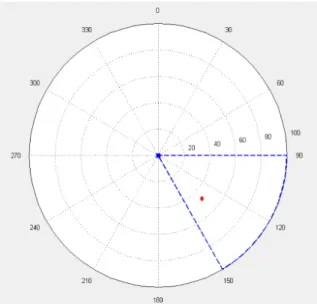
In our radar model, search, track, and MFR modes are provided. The search mode indicates a radar operation that obtains target information with
considerations of elevation coverage, azimuth coverage, and scan time of radar systems.
Fig. 4. Search mode in the radar model
Fig. 5. Track mode in the radar model
The track mode indicates a radar operation that obtains target information without considerations of elevation coverage, azimuth coverage, and scan time of radar systems as an antenna direction follows the target.
The MFR mode indicates a hybrid mode of search and
track, and it firstly operates in search mode and switch to track mode after obtaining a target RCS in search mode. Fig. 4 and 5 show GUI designs of search and track mode respectively.
Fig. 6. Processes of the radar model[1]
Fig. 6 illustrates the processes of our radar model.
The objective of the radar model is to obtain a data set:
observed longitude, latitude and altitude of a target at current simulation time. The radar performance model consists of seven phases in two calculations, two computations, and three models; ① Azimuth, Elevation, and Slant Range Calculation, ② Real RCS Computation,
③ Detection Range Computation, ④ Azimuth and Elevation Coverage Calculation, ⑤ RCS Estimation Model, ⑥ Line Of Sight Model, and ⑦ Longitude Latitude and Altitude Estimation Model. The calculation means an acquisition of values with a single equation.
The computation means an acquisition of values with various equations, more complex than calculations. The
model means an acquisition of values using an independent software module for certain computations.
First, the calculations of azimuth, elevation and slant range are obtaining relative azimuth, elevation, and distances from our radar position to a target position in 3 dimensions. Equation (1) shows expressions for a relative azimuth angle from the radar to a target.
×
,
× (1)
where, TLat = latitude of a target, TLon = longitude of a target,
CRwgs84 = curvature ratio in WGS-84[5] ellipsoid model.
Equation (2) shows expressions for a relative elevation angle from the radar to a target.
×
,
× (2)
where, TAlt = altitude of a target,
GRToTarget = ground range from the radar to a target,
CRwgs84 = curvature ratio in WGS-84[5] ellipsoid model.
Equation (3) shows expressions for a slant range from the radar to a target.
× ×
×
× (3)
where, SRToTarget = slant range from the radar to a target, TLat = latitude of a target,
TLon = longitude of a target, TAlt = altitude of a target, RLat = latitude of the radar, RLon = longitude of the radar,
RAlt = altitude of the radar,
CRwgs84 = curvature ratio in WGS-84[5] ellipsoid model.
Second, the computation of real RCS of a target indicates interpretations of an inputted table data from measured target RCS data sampled in vertical and horizontal degrees in accordance with relative azimuth and elevation angles of the radar to a target and posture data of the target at current simulation time. Fig. 7 visualizes an example of posture data of a target in GUI in our radar model. In this phase, RCS data of a target is finally interpolated within the sampled table data after calculating RCS viewpoints. Equation (4) and (5) show an expression for RCS viewpoint calculations in vertical and horizontal dimensions.
(4)
where, TYaw = yaw degree of a target,
AZRelative = relative azimuth degree to a target (Equation 1)
(5)
where, TPtich = pitch degree of a target, altitude of a target,
ELRelative = relative elevation degree to a target (Equation 2)
Third, the computation of detection range of the radar indicates defining the maximum detection range per RCS in the radar system and determining a target is located in the detection range or not. For this phase, we have adopted Shnidman’s equation[4] for minimum SNR using input parameters such as probability of detection, probability of false alarm, no. of pulse, and swerling no.
We also adopted maximum theoretical range estimate model[4] in MATLAB using input parameters such as wavelength (m), pulse width (sec.), system losses (dB), noise temperature (k), observed RCS (m2), gain (dB), peak transmit power (watt), and minimum SNR from Shnidman’s equation. All maximum detection ranges per
RCS are limited within the maximum radar coverage that is defined in a specification of a target radar system. In this phase, the radar model defines that a target is not detectable at current simulation time if a target is out of range in the radar detection range.
Fig. 7. Posture visualization of a target
Fourth, the calculation of azimuth and elevation coverages of the radar is designed for search mode, not track mode. In this phase, the radar model calculates minimum azimuth/elevation angles and maximum azimuth/elevation angles at current simulation time according to its scan time. Then, the model determines whether a target is in its coverages with relative azimuth and elevation to the target, resulted from azimuth, elevation, and slant range calculation phase. In the following three subsections, we discuss the remaining three models in our radar model.
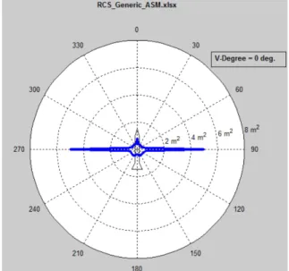
3.3 RCS Estimation Model
In RCS estimation model, we use table data that were actually measured for estimation errors with real slant range and real RCS data. We interpolate an estimation error within the table data after obtaining real slant range and real RCS data at current simulation time. We finally use a random function with lognormal distribution[9] with 0 for mean and ratio of the interpolated estimation error for standard deviation, and
we apply it to the real RCS data. Fig. 8 and 9 depict examples of 2D/3D RCS data. The RCS data in Fig 8 and 9 describe the generic ASM model in Ship Air Defense Model (SADM)[3]. In Section 4, we will conduct a case study with the ASM model as a target.
Fig. 8. An example of 2D RCS data of a target
Fig. 9. An example of 3D RCS Data of a target
3.4 L. O. S. Model
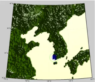
The LOS is an abbreviation for Line Of Sight. In LOS model, we conduct line of sight analysis within selected area of map and elevation data and with relative azimuth and elevation angles from the radar to a target at current simulation time. Fig. 10 shows DTED Level 1 of Korean peninsula[7] displayed in GUI of the radar model.
Fig. 10. An example of L. O. S. visibility analysis
In the radar model, map and elevation data are automatically selected based on geographical locations of the radar model. The circle in figure 10 indicates the radar detection coverage by calculating as one degree of longitude = 88.000 km and one degree of latitude = 112.000 km.
The dark zone inside the circle in figure 10 depicts areas of LOS in viewpoints of the radar, and these areas are computed based on the DTED near the radar, the radar altitude, and a target altitude. In other words, the radar may not detect flying objects because of the terrain even if they are in the green circle.
3.5 LLA Estimation Model
The LLA is an abbreviation for Latitude, Longitude and Altitude. In LLA estimation model, we use table data that were actually measured for slant range errors, azimuth errors, and elevation errors with real slant range
and real RCS data. We interpolate each error within the table data after obtaining real slant range and real RCS data at current simulation time.
We finally use a random function with uniform distribution[10] by setting a minus interpolated result for lower limits and a plus interpolated result for upper limit, and then we apply these errors to the real LLA data. Equation (6), (7), and (8) show expressions for estimated LLA calculations respectively.
,
,
,
× cos × sin ,
,
× (6)
where, SRobserved = observed slant range to a target, SRToTarget = slant range from the radar to a target, ErrorSlantRange = error in slant range,
ELobserved = observed elevation degree to a target, TEl.InRadian = elevation in radian of a target, ErrorEl.InRadian = elevation error in radian, Azobserved = observed azimuth degree to a target, TAz.InRadian = azimuth in radian of a target, ErrorAz.InRadian = azimuth error in radian, DM.P.Lat. = a degree in meter per latitude
(111,200 meter),
LatR.InCurrentTime = latitude of the radar in current simulation time,
CRwgs84 = curvature ratio in WGS-84[5] ellipsoid model.
,
,
,
× cos × cos,
,
× (7)
where, SRobserved = observed slant range to a target, SRToTarget = slant range from the radar to a target, ErrorSlantRange = error in slant range,
ELobserved = observed elevation degree to a target, TEl.InRadian = elevation in radian of a target, ErrorEl.InRadian = elevation error in radian, Azobserved = observed azimuth degree to a target, TAz.InRadian = azimuth in radian of a target, ErrorAz.InRadian = azimuth error in radian, DM.P.Lon. = a degree in meter per longitude
(88,800 meter),
LonR.InCurrentTime = longitude of the radar in current simulation time,
CRwgs84 = curvature ratio in WGS-84[5] ellipsoid model.
,
,
× sin ,
× (8)
where, SRobserved = observed slant range to a target, SRToTarget = slant range from the radar to a target, ErrorSlantRange = error in slant range,
ELobserved = observed elevation degree to a target, TEl.InRadian = elevation in radian of a target, ErrorEl.InRadian = elevation error in radian, AltR.InCurrentTime = altitude of the radar in current
simulation time,
CRwgs84 = curvature ratio in WGS-84[5] ellipsoid model.
3.6 Interoperable with SIMDIS and Exporting Radar Log Data
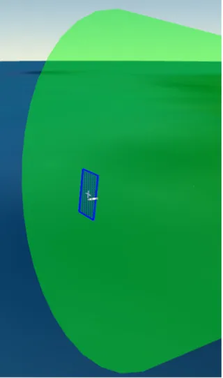
The radar model at the end generates ASCII Scenario Input (ASI) files of SIMulation DISplay (SIMDIS)[6] for visual analyses of the radar. Fig. 11 shows an example of visual verifications in SIMDIS. The green right indicates a radar beam where beam widths are azimuth and elevation coverage of the radar. The blue rectangle indicates a radar gate where gate width is azimuth error, gate height is elevation error, and range gate area is a
coverage in slant range error. In Fig. 11, the target (missile model) is ‘polaris_a-3.opt’ file which is freely provided by SMIDIS.
The radar model also reports radar log data by exporting them in an excel file. All analyzed data such as ground range, slant range, RCS fluctuation, longitude, latitude, and altitude of an observed target are described in response to each of sampled simulation time.
Fig. 11. An example of visual verifications in SIMDIS
4. Case Studies
We have designed two case studies to show practicality of our radar model. First of all, we took
target data from the generic ASM model in SADM with our waypoint data; real RCS table data and trajectory data for a certain flight. The trajectory data consist of time (sec.), longitude (deg.), latitude (deg.), altitude (m), yaw (deg.), pitch (deg.), and roll (deg.) that are sampled in 0.01 sec. during the flight. Fig. 12 outlines our case studies.
(a) Scenario A
(b) Scenario B Fig. 12. Our case studies
We located an ASM launcher at Seoul City Hall (Longitude: 126.9779, Latitude: 37.5666, Altitude: 0) in Scenario A and a BM launcher at Pohang seaside (Longitude: 129.4175, Latitude: 36.0311, Altitude: 0).
These missile models aim at the destination points (Longitude: 125.5387, Latitude: 33.3732, Altitude: 0 in Scenario A and Longitude: 130.8666, Latitude: 37.2486, Altitude: 0 in Scenario B). We also fit up our radar model at Jindo (Longitude: 126.2634, Latitude: 34.4868, altitude: 150 meter) and at Ulleungdo (Longitude:
130.8499, Latitude: 37.4931, altitude: 450 meter) with coverage from 10 to 100 km. We model phase array radars both Jindo and Ulleungdo, and these are operated on MFR mode with wavelength 0.1 (m), pulse width 1.00E-05 (sec.), system losses 15 (dB), noise temperature 290 (k), gain 40 (dB), peak transmit power 100,000 (watt), probability detection 81.029 (%), probability false alarm 1.00E-6 (%). no. of pulse 10, and swerling no. 0.
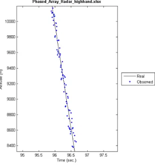
Fig. 13 provides results in the case studies in comparing real trajectory data with observed data from our radar model in views of ground/slant range, RCS measurement, and LLA aspects. In Scenario A, the ASM object came up to the radar system until 94.87 sec. and then gradually became far away. The target had exposed to our radar model from 92.41 to 97.05 sec. (the ASM RCS exposure time during the simulation time). During the exposure time, RCS fluctuation of the ASM object ranged from -5.1 to -2.5 dBsm, and the average of slant range error was 0.953 meter. In Scenario B, the BM object continuously approached to the radar system, and it had exposed to the radar system from 171 sec.
During the exposure time, RCS fluctuation of the missile object ranged from -4.9 to -2.7 dBsm, and the average of slant range error was 1.062 meter.
With those results, we could compare them in views of RCS exposure time, RCS fluctuation, and average of slant range error. In other words, we can conclude that less RCS exposure time is the most proper mission planning result in our missile model. Then, higher averages of slant range error and less average of RCS data are most selective mission planning results during the same RCS exposure time.
(a) Time (sec.) vs. Ground Range (km) in Scenario A
(b) Time (sec.) vs. Ground Range (km) in Scenario B
(c) Time (sec.) vs. Slant Range (km) in Scenario A
(d) Time (sec.) vs. Slant Range (km) in Scenario B
(e) Time (sec.) vs. RCS (dBsm) in Scenario A
(f) Time (sec.) vs. RCS (dBsm) in Scenario B
(g) Time (sec.) vs. Longitude (deg.) in Scenario A
(h) Time (sec.) vs. Longitude (deg.) in Scenario B
(i) Time (sec.) vs. Latitude (deg.) in Scenario A
(j) Time (sec.) vs. Latitude (deg.) in Scenario B
(k) Time (sec.) vs. Altitude (m) in Scenario A
(l) Time (sec.) vs. Altitude (m) in Scenario B
Fig. 13. Results in our case studies
5. Conclusion
In this paper, we have proposed a radar performance model for air defense in guided missile simulations. In previous works, radar systems in M&S focused on functionalities and considerations in real world as many as possible and are attempted to reproduce them in computer systems. However, radar systems themselves become complicated, and results from their radar simulations are critically depended on academical radar equations.
In this paper, we focused on radar systems for air defenses, and we attempted to design our radar performance model to be a simple model and feasible to visual verifications. In the design of our radar model, we have carried out reducing gaps between simulation data and real world data in mission level analyses of our missile model. Finally, we have proved the practicality of our radar performance model through the case studies.
For the future works, we plan to define functionality of seeker performance model in our missile behavior model. At the conclusion, we design and implement the seeker model in M&S that is completely operated by measured performance data in real world like our radar performance model in this paper.
References
[1] Jingyu Kim, “Design of the Radar Performance Model for Mission analyses of Missile Models,”
KIMST Fall Conference Proceedings, pp. 447-448, 2016.
[2] Jingyu Kim, “HLA/RTI based on the Simulation Composition Technology,” Journal of the KIMST, Vol. 19, No. 2, pp. 244-251, 2016.
[3] BAE SYSTEMS, SADM-AE USER’S Guide, Vol.
1: Theory, Australia Ltd. 2012.
[4] Bassem R. Mahafza, Radar System Analysis and Design Using MATLAB, CHAPMAN & HALL/
CRC, 2000.
[5] Sandwell, David T., Reference Earth Model-WGS84, 2002(accessed via topex.ucse.edu/geodynamics/).
[6] U. S. Naval Research Laboratory, SIMDIS User Manual. Visualization System Integration Section.
Code 5773, 2012.
[7] The MathWorks, Mapping Toolbox For Use with MATLAB, User’s Guide Version 2, The MathWorks Inc., 2004.
[8] Roger Aarenstrup, Managing Model-Based Design, The MathWorks Inc, 2015.
[9] M. D. Pretty, R. W. Franceschini, J. Panagos,
“Multi-Resolution Combat Modeling,” In Engineering Principles of Combat Modeling and Distributed Simulation, Edited by A. Tolk, pp. 607-640, John Wiley & Sons, 2012.
[10] Morris R. Driels, “Introduction to Statistical Methods,” In Weaponeering Conventional Weapon System Effectiveness, Second Edition, America Institute of Aeronautics and Astronautics(AIAA), 2013.
[11] Teledyne Brown Engineering Inc., User’s Manual EXTENTED AIR DEFENSE SIMULATION (EADSIM), Ver. 16.00, 2010.