Statistical Inference Concerning Peakedness Ordering between Two Symmetric Distributions

2004, Vol. 15, No. 1 pp. 201-210

Statistical Inference Concerning Peakedness Ordering between Two Symmetric Distributions

Myongsik Oh¹⁾

Abstract

The peakedness ordering is closely related to dispersive ordering. In this paper we consider the statistical inference concerning peakedness ordering between two arbitrary symmetric distributions. Nonparametric maximum likelihood estimates of two distribution functions under symmetry and peakedness ordering are given. The likelihood ratio test for equality of two symmetric discrete distributions in the sense of peakedness ordering is studied.

Keywords : Chi-bar-square, Isotonic regression, Peakedness ordering, stochastic ordering, Symmetry.

1. Introduction

The peakedness ordering has been proposed first by Birnbaum (1948). Let X and Y be two random variables with distribution functions F and G that are symmetric about μ_X and μ_Y, respectively. Then X is said to be smaller than Y in the peakedness ordering if, for every x>0,

(1.1) F( x + μ_X) - F( - x + μ_X) ≥ G( x + μ_Y) - G( - x + μ_Y).

We denote it by X ꀃpeak Y. It is also said that X is more peaked about μ_X than Y about μ_Y. This peakedness ordering is closely related to dispersive ordering.

El Barmi and Rojo (1996) proposed the likelihood ratio test for equality of two distributions against (1.1) in multinomial population. Oh (2003) extended El Barmi and Rojo's estimation procedure to the case of arbitrary distributions and proposed 1) Associate Professor, Department of Statistics, Pusan University of Foreign Studies, Busan, 608-730, Korea

E-mail : [email protected]

the likelihood ratio test for equality of two distributions in the sense of peakedness ordering against (1.1). Their works, however, did not assume that the distributions should be symmetric. In this paper we assume that two distributions are symmetric about known location point, typically mean or median.

Let H_i,i = 0,1,2, be three hypotheses such that

H₀ : F and G are symmetric and F =_peak G, H₁ : F and G are symmetric and F ꀃ_peak G, and H₂ : F and G are symmetric .

where =peak means that equality in (1.1) holds for every x. Note that this does not necessarily imply that F=G. In this paper we are interested in the estimation of F and G under H1 and likelihood ratio tests concerning these hypotheses.

In section 2 we are going to find nonparametric maximum likelihood estimator (NPMLE) of F and G under symmetry and peakedness ordering. In section 3, likelihood ratio tests for equality in peakedness ordering against various alternatives. In section 4, a real data is analyzed for illustrative purpose.

2. Constrained Estimation

Let F and G be distribution functions with symmetric about known location points, μX and μY, respectively. Without loss of generality we assume that μ_X= μ_Y= μ and both random samples are observed at - ∞< t₁< t₂< … < t_k< ∞.

Let δ_1i ( δ_2i) be the number of observations from F(G) at t_i. The ordinary NPMLE of F and G in Kiefer and Wolfowitz's sense maximize

(2.1)

∏

k

i = 1[F(t_i)-F(t_i-)] ^δ1i[G(t_i)-G(t_i-)]^δ2i. Our problem is to maximize (2.1) under H1.

Consider imaginary data points t_{i + k}= 2μ-t_i with δ_{1, i + k}= δ_{2, i + k}= 0 for i = 1,…,k. Let -∞< s₁< s₂< … < s_ℓ≤s_{ℓ + 1}< … < s_2ℓ< ∞ be ordered distinct values of t_i except the case that μ is equal to one of t_i's so that μ=s _ℓ=s_{ℓ + 1}. We observe that ℓ≤k, s_ℓ< μ < s_{ℓ + 1} ( or possibly s_ℓ= μ = s_{ℓ + 1} ) and s_i= 2μ-s_{2ℓ - i + 1}, for i = 1,…,ℓ. For j = 1,…,2ℓ, let

d_1j= ∑

i∈ {1,2,…,2k }:ti=sj

δ_1i and d_2j= ∑

i∈ {1,2,…,2k }:ti=sj

δ_2i. Then (2.1) can be rewritten as

(2.2)

∏

2ℓ

i = 1{F( s_i)-F(s_i-) }^d1i{G( s_i)-G(s _i-) } ^d2i.

The peakedness ordering (1.1) can be expressed as, for j = 0,…,ℓ-1,

(2.3) F( s_{ℓ + 1 + j}) - F( s_{ℓ - j}-) ≥ G( s_{ℓ + 1 + j}) - G( s_{ℓ - j}-).

Now we are going to find F and G which maximize (2.2) subject to H1. This can be achieved by a one-to-one transformation of parameter space. First assume that no observation is equal to μ, i.e., sℓ< μ < s _{ℓ + 1}. For i = 1,…,ℓ, define

p_i= F( s_{ℓ + i})-F(s _{ℓ + i - 1}-), p_{- i}= F( s_{ℓ - i + 1})-F(s_{ℓ - i}-), m_{- i}= d1, ℓ - i + 1, m_i= d_{1, ℓ + i}.

Also define q_i, q_{- i}, n_{- i} and n_i similarly from G. Let p₀= q₀= 0 and m₀= n₀= 0. For the case that at least one observation is equal to μ, i.e., s_ℓ= μ = s_{ℓ + 1}, let p₀= F( s_{ℓ + 1}) - F( s_ℓ-), q₀= G( s_{ℓ + 1}) - G( s_ℓ-), m₀= d_{1, ℓ}+d_{1, ℓ + 1}, and n0= d_{2, ℓ}+d_{2, ℓ + 1}, and for i = 1,…,ℓ-1,

p_i= F( s_{ℓ + i + 1})-F(s_{ℓ + i}-), p_{- i}= F( s_{ℓ - i})-F(s_{ℓ - i - 1}-), m_{- i}= d_{1, ℓ - i}, m_i= d1, ℓ + i + 1.

p_ℓ= q_ℓ= 0 and m_ℓ= n_ℓ= 0. We use the convention 0⁰= 1. Then (2.2) becomes

(2.4) p₀^m0q₀ⁿ⁰∏

ℓ

i = 1[^{pm-i- ipmi iqn-i- iqnii}]

and the restrictions become

p_{- i}= p_i, q_{- i}= q_i for i = 1,…,ℓ, p₀≥q₀, p₀+∑

i

j = 1(p_{- j}+ p_j)≥q₀+∑

i

j = 1(q_{- j}+ q_j) for i = 1,…,ℓ - 1, and p₀+∑^ℓ

j = 1(p_{- j}+ p_j) = q₀+∑^ℓ

j = 1(q_{- j}+ q_j).

Let

S = { x ∈ R^{4ℓ + 2}: x_i= x_{2ℓ + 2 - i}, x_{2ℓ + 1 + i}= x_{4ℓ + 3 - i}, for i = 1,…,ℓ }, C = { x ∈ R^{4ℓ + 2}: x_{ℓ + 1}≥x_{3ℓ + 2},

x _{ℓ + 1}+∑ⁱ

j = 1(x_{ℓ + 2 - i}+x_{ℓ + 1 + i}) ≥ x_{3ℓ + 2}+∑

i

j = 1(x_{3ℓ + 3 - i}+x_{3ℓ + 2 + i}), i = 1,…,ℓ-1, x _{ℓ + 1}+∑

ℓ

j = 1(x_{ℓ + 2 - i}+x_{ℓ + 1 + i}) = x_{3ℓ + 2}+∑

ℓ

j = 1(x_{3ℓ + 3 - i}+x_{3ℓ + 2 + i}) } It is not difficult to show that S is a linear subspace of R^{4ℓ + 2} and C is a closed, convex cone in R^{4ℓ + 2}. Let p and q be the solution to the maximization problem of (2.4) subject to H₁. Then ( p , q ) = E(^{( pˆ, qˆ) | S∩C})^{, where}

E( x|A) is the projection of x onto A. See Robertson, Wright and Dykstra (1988, RWD henceforth) for the details of projection theory. Now we restate the Theorem 5.5.1 of RWD, which plays an important role in estimation.

Lemma If ℒ is a linear subspace of R^k and if ℱ is a closed, convex cone in R^k and if for each x∈R^k, E( E( x|ℒ)|ℱ)∈ℒ∩ℱ, then

E(x|ℒ∩ℱ) = E(E(x|ℒ)|ℱ).

Under the assumption of symmetry, (2.4) can be rewritten as

(2.5) p₀^m0q₀ⁿ⁰∏^ℓ

i = 1[^pmi ^{- i+mi}qⁿ_i^{- i+ni}]

and the peakedness ordering becomes p₀≥q₀, p₀+ 2∑ⁱ

j = 1p_j ≥ q₀+ 2∑ⁱ

j = 1q_j, for i = 1,…,ℓ - 1, and p₀+ 2∑^ℓ

j = 1p_j = q₀+ 2∑^ℓ

j = 1q_j= 1.

The unconstrained solution to (2.5) provide the MLE under symmetry assumption.

Hence the constrained solutions satisfy the peakedness ordering. It follows from Lemma that the constrained solution to (2.5) are the solution to (2.4) under H₁. Now the estimation problem becomes the estimation under usual stochastic ordering, which is studied extensively many researchers. Robertson and Wright (1981) found the closed form of MLE of multinomial parameter under stochastic ordering. By appealing to it we have the following.

Theorem 2.1 If for all i, m_i, n_i> 0 then p₀= m₀

m ⋅E _m

(

)

, q₀= n₀

n ⋅E _n

(

)

, p_i= p_{- i}= 1

2

m_{- i}+m_i

m ⋅E _m

(

)

, q_i= q_{- i}= 1

2

n_{- i}+n_i

n ⋅E _n

(

)

,

where m = ∑^ℓ

i =- ℓm_i, n = ∑^ℓ

i =- ℓn_i, m = ( m_0,m₁+m_{- 1},…,m_ℓ+ m_{- ℓ}), n = ( n_0,n₁+n_{- 1},…,n_ℓ+ n_{- ℓ}), A = { x = ( x₀,…,x_k)∈R^{ℓ + 1} : x₀≥x₁≥…≥x_ℓ}, and A' = { x ∈R^{ℓ + 1} : - x ∈A }, E(⋅|⋅) _i represents the ith component, and all vector operations are componentwise.

In Theorem 2.1 we assume that no missing observations exist. We note that the vectors m and n may contain several components whose values are zero since we use imaginary data points. In this case we can not apply Theorem 2.1 directly to the problem. Lee (1987) studied the estimation problem when some components

of multinomial parameters are random or fixed missing. His idea is collapsing the missing components with the adjacent components without violating the stochastic ordering among the collapsed components and apply Robertson and Wright's estimation procedure. For some cases, however, this estimation procedure may not give unique MLE.

Now we are going to show that the NPMLE given by Theorem 2.1 is strongly consistent. Suppose x < μ and let G and G ˜ be restricted NPMLE of G under H₁ and H2 respectively and ˆG be empirical distribution of G. We note that G depends on both of m and n while ˜G ^and ˆG depend only on n. Let H( t) = G( t + μ) - G(μ - t). Note that H is also a distribution function. Since G is symmetric about known location μ, we have G( x) = (1 -H(μ-x) )/2 and hence we can write

G ( x) - G( x) = G ( x) - G ˜( x )+ G ˜( x )- G( x)

= 1

2 [ H ˆ( μ - x ) -H ( μ - x)] + G ˜( x )- G( x) Note that ˜G ( x )= 1

2 ( G ˆ( x )+ 1 - G ˆ( 2μ - x )) then we have

˜G ( x )- G( x) = 1

2 ( G ˆ( x )+ 1 - G ˆ( 2μ - x )) - 1

2 ( G( x) + 1 - G( 2μ - x))

= 1

2 [ G ˆ( x )- G( x)] - 1

2 [ G ˆ^{( 2μ - x )}- G( 2μ - x)]

→ 0 almost surely.

It is well known that NPMLE of distribution functions under stochastic ordering is strongly consistent. This was proved first by Brunk, Franck, Hansen and Hogg (1966) and the refinement of their proof can be found in Dykstra, Kochar and Robertson (1995). It then follows that ˆH ( μ - x ) -H ( μ - x) → 0 uniformly (almost surely). Since G is symmetric G ˆ( x ) - G ( x ) → 0 almost surely for x > μ.

By similar argument we also can show that ˆF ( x ) - F ( x ) → 0 uniformly. Now we have the following theorem.

Theorem 2.2 The constrained NPMLEs F and G converges uniformly to F and G almost surely, respectively, as m and n go to infinity provided that

F ≤_peak G.

Under H₀ the constrained NPMLE of distribution functions can be easily obtained. We need to maximize (2.4) subject to

p_{- i}= p_i, q_{- i}= q_i for i = 1,…,ℓ,

p₀= q₀, p_{- j}+ p_j= q_{- j}+ q_j for i = 1,…,ℓ.

This maximization problem is equivalent to maximize (2.5) subject to

p₀= q₀, p_j = q_j for j = 1,…,ℓ.

Now we have

p^o₀= q^o₀= m₀+n₀

m+n ,

p^o_{- j}= p^o_j= q^o_-j= q^o_j= m_{- j}+ m_j+ n_{- j}+n_j

m+n .

3. Likelihood Ratio Tests

Assume that F and G have the same support on the fixed index set { - ℓ, …, - 1, 0,1,…,ℓ } and each point has positive probability, so that we are concerned with discrete distribution with common support. In this section we consider the test of equality in peakedness of two discrete distributions against a peakedness ordering. The likelihood ratio test for testing H0 against H1-H₀ rejects for sufficiently large values of

T₀₁= 2 ∑^ℓ

i =- ℓm _i( ln p_i- ln p^o_i) + 2 ∑^ℓ

i =- ℓn_i( ln q_i- ln q^o_i).

Now we derive the asymptotic null distribution of T₀₁. T ₀₁ = 2m₀( ln p₀- ln p^o₀) + 2∑^ℓ

i = 1(m_{- i}+m _i)( ln 2 p_i- ln 2p^o_i) + 2n ₀( ln q₀- ln q^o₀) + 2∑

ℓ

i = 1(n_{- i}+n _i)( ln 2 q_i- ln 2q^o_i).

Note that ( p₀,2p₁,…,2p_ℓ) and ( q₀,2q₁,…,2q_ℓ) are two multinomial parameters. Careful review of T01 reveals that it is just a test statistic for testing equality of two multinomial parameters (p₀,2p₁,…,2p_ℓ) and ( q₀,2q₁,…,2q_ℓ) against stochastic ordering, specifically

p_o≥q₀, p₀+∑

i

j = 12p_j ≥ q₀+∑

i

j = 12q_j for i = 1,…,ℓ - 1, and p₀+∑^ℓ

j = 12p_j = q₀+∑^ℓ

j = 12q_j= 1.

Appealing to Theorem 4.1 of Robertson and Wright (1981) or Theorem 5.4.5 of RWD we have the following Theorem.

Theorem 3.1 If F =peak G then for each real t,

m, n→∞lim Pr[T₀₁≥t] = ∑

ℓ

i = 0P _S(i,ℓ+1;( p ₀,2p₁,…,2p_ℓ)) Pr [χ²_{ℓ - i}≥t]

≤ 1

2 [^{Pr [χ2}ℓ≥t] + Pr [χ²_{ℓ - 1}≥t]]^,

where P_S(i,ℓ+1;( p₀,2p₁,…,2p_ℓ)) is the level probability with respect to simple ordering and weights (p0,2p₁,…,2p _ℓ).

The distribution associated with the maximum right-tail probability in Theorem 3.1 is called least favorable distribution. One might use this least favorable distribution to find a critical value since the asymptotic null distribution of T₀₁ depends upon the unknown weights ( p₀,2p₁,…,2p_ℓ). This test is, however, likely to be very conservative. To resolve this difficulty one may use an estimate of weights to approximate the asymptotic null distribution. This generally provides a quite reasonable approximation. An alternative method such as equal-weight approximation of level probability could be used. For the comprehensive discussion of this problem can be found in Chapter 3 of RWD.

If we assume that F and G have the same support on the fixed index set { - ℓ, …, - 1, 1,…,ℓ }, then the likelihood ratio test for testing H₀ against H₁-H₀ rejects for sufficiently large values of

T^'₀₁= 2 ∑^ℓ

i =- ℓ,i≠0m _i( ln p_i- ln p^o_i) + 2 ∑^ℓ

i =- ℓ,i≠0n _i( ln q_i- ln q^o_i).

To find a critical value one may use the following theorem.

Corollary 3.2 If F =peak G, then for each real t,

m, n→∞lim Pr[T^'₀₁≥t] = ∑^ℓ

i = 1P_S(i,ℓ;( p₁,…,p _ℓ)) Pr [χ²_{ℓ - i}≥t]

≤ 1

2 [^{Pr [χ2}ℓ - 1≥t] + Pr [χ²_{ℓ - 2}≥t]]^.

As a goodness-of-fit test one might be interested in testing peakedness ordering against all alternative with symmetry assumption. That is, we consider the test of H₁ against H2- H₁. Assume first that F and G have the same support on the fixed index set { -ℓ,…,-1,0,1,…,ℓ }. The likelihood ratio test for testing of

H₁ against H2- H₁ rejects for large values of T₁₂ = 2 ∑

ℓ

i =-ℓm_i( ln p˜_{i- ln qi) +2 ∑}^ℓ

i =-ℓn_i( ln q˜_{i- ln qi)}

= 2m₀( ln p˜_{0- ln p}ˆ₀) + 2∑^ℓ

i = 1(m_{- i}+m_i)( ln 2 p˜_{i- ln 2 p}ˆ_i) + 2n ₀( ln q˜_{0- ln q}ˆ₀) +2∑^ℓ

i = 1(n_{- i}+n _i)( ln 2 q˜_{i- ln 2 q}ˆ_i).

Appealing to Theorem 4.2 of Robertson and Wright (1981) or Theorem 5.4.6 of RWD we have the following Theorem.

Theorem 3.3 If F ≤peak G then for each real t, sup_F≤peakG lim

m, n→∞Pr[T₁₂≥t] = sup_{F =peakG} lim

m, n→∞Pr[T₁₂≥t]

= ∑^ℓ

i = 0

ℓ

( )

A critical value for a conservative test for testing H₁ against H₂- H₁ can be obtained from Theorem 3.2. If less conservative test has to be used see Oh (1994).

If we restrict F and G on the fixed index set {-ℓ,…,-1,1,…,ℓ }, then the likelihood ratio test for testing H₁ against H₂- H₁ rejects for sufficiently large values of

T^'₁₂= 2 ∑^ℓ

i =- ℓ,i≠0m_i( ln p˜_{i- ln p}ˆ_i) + 2 ∑^ℓ

i =- ℓ,i≠0n_i( ln q˜_{i- ln q}ˆ_i).

To find a critical value for a conservative test we may use the following theorem.

Corollary 3.4 If F =_peak G, then for each real t, sup_F≤peakG lim

m, n→∞Pr[T^'₁₂≥t] = sup_{F =peakG} lim

m, n→∞Pr[T^'₁₂≥t]

= ∑^ℓ

i = 1

ℓ-1 i - 1

( )

In theorems 3.3 and 3.4, only the least favorable distributions are given.

Approximations to the exact asymptotic null distributions of T12 and T^'₁₂ are available, but it is not easy to use them since the way the distribution depend on unknown weights are quite complicated. Interested readers may refer to Oh (1994).

If the underlying distributions are arbitrary, especially continuous, the null distributions of likelihood ratio test statistics are extremely complicated and hence the application of the above results may restricted severely. Dykstra, Madsen, and Fairbanks (1982) studied a nonparametric likelihood ratio test and provided the critical values for various selections of sample sizes m and n. On the other hand, if the sample sizes are relatively small we may use the theorems given in this sections to find critical values.

4. An Illustrative Example

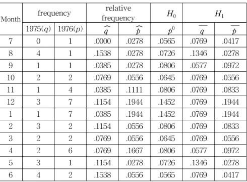
We analyze a real data to illustrate the inferential procedure proposed in this paper. The following table lists the frequencies of trisomy among karyotyped spontaneous abortions of pregnancies by calendar month of the last menstrual period for the months July to June of 1975 and 1976. The complete data may be found in Tango (1984) or data set 197 of Hand et

al. (1994). We are interested in testing the equality of two distribution in the sense of peakedness ordering. Note that the peakedness is compared about the end of December or the first of January. The following table shows the computational details of two distributions under H0 and H1.

Table 1. Computational details.

Month frequency relative

frequency H₀ H₁

1975(q) 1976(p) ˆq ˆ_{p p}⁰ _{q p}

7 0 1 .0000 .0278 .0565 .0769 .0417

8 4 1 .1538 .0278 .0726 .1346 .0278

9 1 1 .0385 .0278 .0806 .0577 .0972

10 2 2 .0769 .0556 .0645 .0769 .0556

11 1 4 .0385 .1111 .0806 .0769 .0833

12 3 7 .1154 .1944 .1452 .0769 .1944

1 1 7 .0385 .1944 .1452 .0769 .1944

2 3 2 .1154 .0556 .0806 .0769 .0833

3 2 2 .0769 .0556 .0645 .0769 .0556

4 2 6 .0769 .1667 .0806 .0577 .0972

5 3 1 .1154 .0278 .0726 .1346 .0278

6 4 2 .1538 .0556 .0565 .0769 .0417

The value of likelihood ratio test statistic is 9.3976. To find p-value for this example we consider three cases. First we consider the test based on the least favorable distribution. The computed p-value is

( Pr [χ²_{6 -1}≥9.3976] + Pr [χ²_{6 -2}≥9.3976])/2 = 0.0731.

Second, we use equal-weight level probability. The level probabilities are 0.1667, 0.3806, 0.3125, 0.1181, 0.0208, and 0.0014 and hence the p-value based on equal-weight approximation is 0.0442. Finally we use approximation of level probability using the algorithm given by Pillers, Robertson and Wright (1984). The computed level probabilities are 0.1835, 0.3931, 0.2987, 0.1057, 0.0178, and 0.0011 and hence the p-value 0.0459.

References

1. Brunk, H. D., Franck, W. e., Hanson, D.L., and Hogg, R. V. (1966).

Maximum likelihood estimation of the distributions of two stochastically

ordered random variables, Journal of the American Statistical Association, 61, 1067-1080.

2. Dykstra, R. L., Kochar, S. C., and Robertson, T. (1995). Likelihood ratio tests for symmetry against one-sided alternatives, Annals of Institute of Statistical Mathematics, 47, 719-730.

3. Dykstra, R. L., Madsen, R. W., and Fairbanks, K. (1982) . 　A

nonparametric likelihood ratio test,　 Journal of Statistical Computation and Simulation, 18, 247-64.

4. El Barmi, H. and Rojo. J. (1996). Likelihood ratio tests for peakedness in multinomial populations, Journal of Nonparametric Statistics, 7, 221-237.

5. Hand, D. J., Daly, F., Lunn, A. D., McConway, K. J., and Ostrowsky, E. (1994).

A Handbook of Small Data Sets, Chapman & Hall, London.

6. Lee, C. I. C. (1987). Maximum likelihood estimates for stochastically ordered multinomial populations with fixed and random zeros,

Foundation of Statistical Inference (I. B. MacNeill and G. J. Umphrey eds.), 189-197.

7. Oh, M. (1994). Statistical Tests Concerning a Set of Multinomial Parameters under Order Restrictions: Approximations to Null Hypotheses Distributions, Ph. D. Thesis, The University of Iowa.

8. Oh, M. (2003). Inference for peakedness ordering between two distributions. Unpublished manuscript.

9. Pillers, C., Robertson T., and Wright F. T. (1984). A FORTRAN program for the level probabilities of ordered restricted inference, Journal of the Royal Statistical Society (C), 33, 115-119.

10. Robertson, T. and Wright, F. T. (1981). Likelihood ratio tests for and against a stochastic ordering between multinomial populations, The Annals of Statistics, 9, 1248-1257.

11. Robertson, T., Wright, F. T., and Dykstra, R. L. (1988). Order Restricted Statistical Inference, Wiley, Chichester.

12. Tango, T. (1984). The detection of disease clustering in time, Biometrics, 40, 15-26.

[ received date : Sep. 2003 , accepted date : Dec. 2003 ]