A Practical FastSLAM Implementation Method using an Infrared Camera for Indoor Environments

(1)

실내 환경에서 Infrared 카메라를 이용한 실용적 FastSLAM 구현 방법

A Practical FastSLAM Implementation Method using an Infrared Camera for Indoor Environments

장 헤 이 롱

¹

, 이 헌 철

²

, 이 범 희

³

Zhang Hairong

¹

, Lee Heon-Cheol

²

, Lee Beom-Hee

³

Abstract FastSLAM is a factored solution to SLAM problem using a Rao-Blackwellized particle filter. In this paper, we propose a practical FastSLAM implementation method using an infrared camera for indoor environments. The infrared camera is equipped on a Pioneer3 robot and looks upward direction to the ceiling which has infrared tags with the same height. The infrared tags are detected with theinfrared camera as measurements, and the Nearest Neighbor method is used to solve the unknown data association problem. The global map is successfully built and the robot pose is predicted in real time by the FastSLAM2.0 algorithm. The experiment result shows the accuracy and robustness of the proposed method in practical indoor environment.

Keywords : SLAM, FastSLAM2.0, Infrared Camera, Unknown Data Association

1. Introduction¹⁾

The problem of Simultaneous Localization and Mapping, also known as SLAM, is one of the main topics in the robotics. The goal of SLAM is to construct a map of the environment and the path taken by the robot.

SLAM is considered as a key prerequisite for truly autonomous robots. FastSLAM, which uses a Rao- Blackwellized particle filter, factors the SLAM posterior into a product of a robot path posterior and landmark posterior conditioned on the robot path estimate

^[1]

. The factorization allows advantages to FastSLAM over Extended Kalman Filter SLAM (EKF-SLAM) on two aspects: computation complexity and robust data association.

Received: Sep. 30. 2009; Reviewed: Nov. 16. 2009; Accepted: Nov. 23. 2009

※ 본 연구는 BK21과 교육과학기술부 NRL 프로그램(No. R0A-2008-000- 20004-0), 지식경제부 성장동력기술개발사업, 서울대학교 자동화시스 템공동연구소(ASRI)의 연구 지원으로 수행되었음.

1

삼성전자DMC사업부 연구원

2

서울대학교 전기컴퓨터공학부 박사과정

3

서울대학교 전기컴퓨터공학부 교수

FastSLAM experiment is usually implemented using odometry sensor for motion input and observation sensors such as sonar, laser and camera. More recently, Davison

^[12]

proposed a vision-based real-time SLAM, called Mono-SLAM, which employs only a single camera without odometry information. It increases localization accuracy by integrating camera velocity into optimization variables. However, it needs an initial manual calibration process to obtain the scale information. In [4], Jeong et al.

proposed a CV-SLAM (Ceiling Vision–based Simultaneous Localization and Mapping) technique using a single ceiling vision sensor, which was suitable for system that demands very high localization accuracy. A single camera looking upward direction was mounted on the robot, and salient image features were detected and tracked through the image sequence. Compared with the conventional frontal view systems, their method had advantage in tracking, since it involved only rotation and affine transform without scale change.

However, a common camera cannot ensure reliable

(2)

performance when illumination condition is not good, e.g.

in a dark room. In order to solve this problem, this paper proposes to use an infrared camera instead of a common camera as the observation sensor in FastSLAM experiment. The proposed observation method can not only overcome the bad illumination condition, but also can be implemented much easier. A single infrared camera looking upward direction was mounted on the Pineer3 robot, and IR tags on the ceiling of an Intelligent Space were detected by the infrared camera. The proposed method used the Nearest Neighbor method to solve the unknown data association problem and was implemented using Visual C++ for the real-time processing. The results of the proposed method showed lower errors in the robot pose and the map built by the robot.

The layout of this paper is as follows. Section 2 describes FastSLAM with unknown data association. In Section 3, the infrared camera is proposed, and its measurement model is built. Section 4 shows the practical indoor experiments of FastSLAM with an infrared camera, and their results arecompared with global vision result. At last, Section 5 gives conclusion.

2. FastSLAM with Unknown Data Association

2.1 FastSLAM2.0 Algorithm

FastSLAM computes the posterior over maps and robot path as follows:

1: 1: 1: 1:

1: 1: 1: 1: 1: 1: 1: 1:

path posterior 1

landmark estimators

( , | , , )

= ( | , , ) ( | , , , ).

t t t t

N

t t t t n t t t t

n

p s z u n

p s z u n p θ s z u n

=

Θ

1442443

∏

14444244443

(1)

This factorization states that the SLAM posterior can be separated into a product of robot path posterior

1: 1: 1: 1:

(

_t

|

_t

,

_t

,

_t

)

p s z u n , and N landmark posteriors conditioned on the robot’s path. Here s

1:t

means robot path, Θ means the set of all n landmark positions, z

1:t

means sensor observation, u

1:t

means robot control input, n

1:t

means the data association of observation

[5, 10, 11]

.

In this paper, we implement the FastSLAM2.0 algorithm, which draw a new pose s

t

from a motion model that includes the most recent observation z

t

.

[ ] [ ]

1: 1 1: 1: 1:

( | , , , )

m m

t t t t t t

s = p s s

₋

u z n (2)

where

1: 1^{[ ]} m

s

t₋

is the path up to time t-1 attached to the m-th particle. Motion andmeasurement models are given as nonlinear function with Gaussian noise

^[9]

:

1 1

( | ,

_t _t _t

) (

_t

, )

_t _t

p s u s

₋

= h s

₋

u +

δ

(3)

( | , , )

_t _t _t

( ,

_t _n_t

)

_t

p z s Θ n = g s

θ

+

ε

(4) Here g and h are nonlinear functions, and

ε_t

and δ

_t

are independent Gaussian noise. A particle at time t, S

t^{[ ]}^k

in FastSLAM is denoted by

[ ] [ ] [ ] [ ] [ ] [ ]

1, 1, , ,

, , , , ,

k k k k k k

t t t t N t N t

S = s μ Σ K μ Σ (5)

where the [k] indicates the index of the particle, and

[ ]k

S is the pose estimate of the robot at time t. Only the

t

most recent pose S is used in FastSLAM, so a particle

t^{[ ]}^k

keeps only the most recent pose. μ

_{n t}^{[ ]}^k,

, Σ

^{[ ]}_{n t}^k,

are mean and covariance of the Gaussian, representing the n-th feature location relative to the k-th particle, respectively.

Altogether, these elements form the k-th particle, S , and

t^{[ ]}^k

there are total M particles and N feature estimates in a particle set. The basic steps of the FastSLAM 2.0 algorithm, which is the latest version, are as follows

^[13]

:

• Step 1: Sampling. s

_t^{[ ]}^k

~ ( | p s s

_t ^{[ ]}_t₋^k1

, , , ) z u n

^t ^t ^t

• Step 2: Measurement update. For each observed feature identify the correspondence j for the measurement z and incorporate the measurement

_tⁱ

z

_tⁱ

into the corresponding EKF by updating the mean

[ ] , k

u

j t

and covariance Σ

^{[ ]}_{j t}^k_,

.

• Step 3: Importance weight. Calculate the importance weight w for the k-th particle.

^{[ ]}^k

• Step 4: Resampling. Sample M particles with replace-

ment, where each particle is sampled with a

probability proportional to w .

^{[ ]}^k

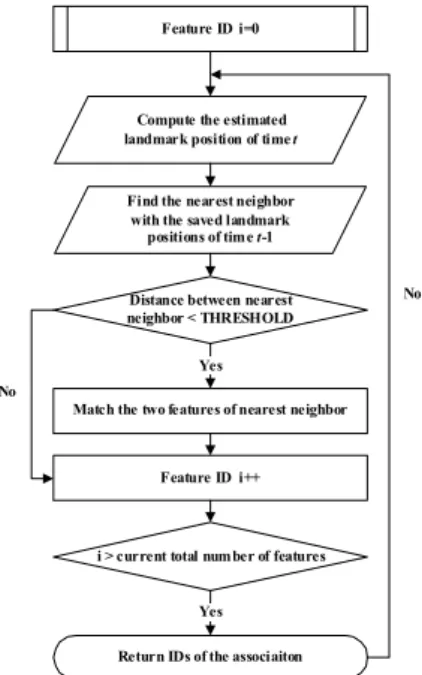
(3)

Feature ID i=0

Compute the estimated landmark position of time t

Find the nearest neighbor with the saved landmark

positions of time t-1

Distance between nearest neighbor < THRESHOLD

Match the two features of nearest neighbor Yes

No

Feature ID i++

i > current total number of features

Yes Return IDs of the associaiton

No

Fig. 1. Nearest Neighbor data association algorithm

2.2 Unknown Data Association

Data association is one of the critical issues for practical SLAM implementations. In practice, the data association is rarely known. Two factors contribute to data association uncertainty in the SLAM posterior:

measurement noise and motion noise. As measurement noise increases, the distributions of possible observations of every landmark become more uncertain. If measurement noise is sufficiently high, the distributions of observations from nearby landmarks will begin to overlap substantially.

This overlap leads to ambiguity in the identity of the landmarks. This kind of data association ambiguity caused by measurement is called as measurement ambiguity. In order to distinguish each feature and solve the data association problem, we implement the Nearest Neighbor method, which is easy and robust in our system as the tags are sparse. Nearest Neighbor data association method is among the simplest of the data association methods.

The basic idea of NN algorithm is to match the two features with the shortest distance of time-adjacent measurements. This algorithm can be applied when the feature distribution is sparse and not very complicate. Fig.

1 in the next page demonstrates the algorithm of Nearest Neighbor data association method. However, the NN data association method may be not stable when the data association problem is very complicate. As the data

association error can induce significant errors in the map, we may implement or develop some more robust data association method to solve this problem.

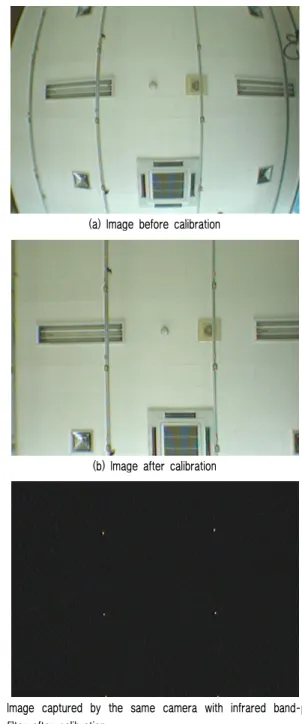
3. Observation using Infrared Camera

The infrared technique is widely used for night vision systems. In this paper, an infrared band-pass filter is covered on a common camera, which transmits only infrared band by filtering out visible band. The infrared tags on the ceiling are well discriminated as white blobs in the image. As is well known in vision community, it is difficult to robustly locate particular patterns from images in varying illumination condition

^{[2, 3]}

. This infrared band-pass filtering solution makes the observation much simpler, and enables this kind of observation at any illumination condition.

Fig. 2 demonstrates the effect of infrared band-pass filter. Fig. 2(a) was captured with a normal camera, Fig.

2(b) was the camera image with calibration, and Fig. 2(c) was captured with the same camera but with an infrared band-pass filter. The infrared tags on the ceiling are easily recognized aswhite blobs in the image. In order to estimate the position of the IR tags in the image plane, let I(x,y) be an image plane. First, the image is converted into a binaryimage by some threshold got by experiments. The white blobs of IR tags are then located by connected component analysis. Let b

i

be the i-th blob, for i = 1,…,n.

Finally, the mass center of each blob, (x

i

, y

i

), is given by

( , )

1 ( , )

i

i i

x y b i

i

x y b i

x x I x y

s

y y I x y

s

∈

= ⋅

∑

∑ ⁽⁶⁾

where ^s

ⁱ

⁼ ∑

_b_i

^{I x y} ^{( , )} , for i = 1, …, n.

Before identifying the infrared spots on the image of the infrared camera, the calibration of camera is a necessary step. In this paper, the established calibration method from Bouguet’s Matlab source was implemented

^{[6, 7]}

.

In the next step, the image projection model will be built up. Projection model is the projection function that projects a 3D landmark to the infrared camera observation.

Our observation system has an infrared camera positioned

(4)

(a) Image before calibration

(b) Image after calibration

(c) Image captured by the same camera with infrared band-pass filter after calibration.

Fig. 2. Observation sample images of infrared tags

Fig. 3. Measurement model: projection from infrared tags onto image plane

Common Camera Calibration Infrared Band-pass Filter

Threshold Selection Image Projection

Fig. 4. General scheme of proposed observation method using infrared camera

at the center of the robot, aligned with the robot orientation. Fig. 3 demonstrates the measurement model which projects from the infrared tags on the ceiling onto image plane. Fig. 4 describesthe general scheme of the proposed observation method using infrared camera.

For the measurement model, we mount the infrared camera at the center of the robot, looking upward direction. The infrared tags are observed with the

following observation model.

2 2

, , , ,

, ,

1

,

, ,

( , )

(( ) ) (( ) )

( , ) ( , )

tan ( )

t t nt

x y

nt x t x nt y t y

t nt z z

t nt nt y t y x

t

nt x t x y

z g s

f f

s s

r s h h

s s f s

s f

^θ

θ

θ θ

θ

φ θ θ

θ

−

=

⎡ ⎤

− ⋅ + − ⋅

⎢ ⎥

⎡ ⎤ ⎢ ⎥

= ⎢ ⎣ ⎥ ⎢ ⎦ ⎢ = − ⋅ − ⎥ ⎥

⎢ − ⎥

⎣ ⎦

(7)

where s

_t

= [ s s s

_{t x}, _{t y}, _t,_θ

] donates robot pose,

, ,

[ ]

nt nt x nt y

θ = θ θ donates current landmark position and f

^y

denotes the focal length of the camera, and h

^z

denotes the

height from the robot to the ceiling. The Jacobians are

computed as follows:

(5)

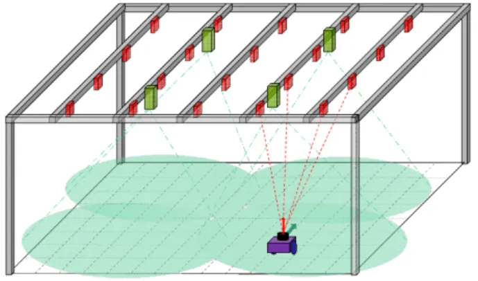
Fig. 5. Intelligent space

Fig. 7. Landmark positions by FastSLAM compared with real landmark positions

, ,

, , , ,

0

1

t

nt y t y

nt x t x

s

nt y t y nt x t x

s s

q q

G s s

q q

θ θ

−

⎡ − ⎤

− −

⎢ ⎥

= ⎢ − − ⎥

⎢ − − ⎥

⎢ ⎥

⎣ ⎦

(8)

where q = ( θ

_{nt x}^,

− s

_{t x}^,

)

²

+ ( θ

_{nt y}^,

− s

_{t y}^,

)

²

.

, ,

, , , ,

nt

nt y t y

nt x t x

nt y t y nt x t x

s s

q q

G s s

q q

θ

θ θ

−

⎡ − ⎤

⎢ ⎥

= ⎢ − − ⎥

⎢ − ⎥

⎢ ⎥

⎣ ⎦

(9)

where q = ( θ

_{nt x}^,

− s

_{t x}^,

)

²

+ ( θ

_{nt y}^,

− s

_{t y}^,

)

²

_.

4. Experiments

4.1 Intelligent Space with Infrared Tags

The Intelligent Space is illustrated in Fig. 5. There are 20 infrared tags (red) and 4 global cameras (green) with the same height h

z

= 2145mm on the ceiling. This is a very important assumption of our experiment. The P3DX mobilerobot is moving on the floor for a close loop with an infrared camera equipped at the center of it. The experiment is done in real-time with Visual C++ program.

In the real environment, the floor is flat, that is to say, the direction camera would keep perpendicular to the floor. However, if the floor is not even, e.g. in outdoor environment, this kind of experiment will probably have bad performance.

4.2 Experimental Results

In the Intelligent Space mentioned in Fig. 5, we did the FastSLAM experiment for more than 10 times. First, we turn off the fluorescent lights in the room, which are not with the same height as infrared tags on the ceiling and may lead to incorrect matching of the measurement. And then, let the Pioneer3 robot go around the room for many closing loops. One of these experiments is demonstrated in the Fig. 6, where the red dots denote the landmarks (infrared tags) on the ceiling, the blue circle denote the current pose of robot by estimation, and the blue polyline denotes the estimated robot trajectory.

Fig. 6. FastSLAM experiment result

4.3 Analysis of the Results

4.3.1 Position error of landmarks

Fig. 7 shows the mapping result by FastSLAM2.0

compared with the real position of tags. The estimated

(6)

Average (mm) Standard Deviation (STD)

50.7 34.8

Table 1. Landmark position error by FastSLAM

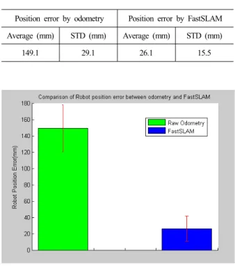
Position error by odometry Position error by FastSLAM Average (mm) STD (mm) Average (mm) STD (mm)

149.1 29.1 26.1 15.5

Table 2. Robot position errors comparison between odometry and FastSLAM

Fig. 8. Robot position error comparison between odometry and FastSLAM

positions of landmarks are represented by red crosses and the real positions with blue circle. Table 1 shows the average value and standard deviation value of landmark position error by FastSLAM.

4.3.2 Position error of the robot

The robot pose can be compared with result of global vision system. Table 2 shows the average values and standard deviation values of robot position error by raw odometry and FastSLAM. Fig. 8 also shows the average values and standard deviation values of robot position error by raw odometry and FastSLAM. The experiment results of the robot position show that the estimated position by FastSLAM was much more accurate than the raw odometry result. This is helpful to localize the robot for other tasks.

5. Conclusion

In this paper, a novel method to implement FastSLAM algorithm was proposed using infrared camera with unknown data association. The proposed method has several advantages over other methods with a common camera as follows:

Regardless of illumination conditions —The proposed method can overcome bad illumination conditions such as too dark or too bright illumination, shiny sunlight, and highly reflective objects, because the IR camera observes only IR light of the environment. Even if in totally dark environment, the proposed IR camera method can successfully perform FastSLAM by observing IR tags consistently.

Less processing time —The proposed method can make the complicated image processing much simpler. The method converts the raw image after undistortion into a binary image, and then searches the bulb with high value (white color) over some threshold by experiment.

Therefore, the method ensures less processing time for observation, because the simpler image processing requires less total processing time.

Finally, the performance of the proposed method was verified by reducing the errors in both the robot position and the map built by the robot compared with raw odometry data. As a future work, we will deal with more realistic environment, e.g. with only fluorescent lights instead of artificial infrared tags, or with both fluorescent lights and infrared tags.

참 고 문 헌

[1] M. Montemerlo, “FastSLAM: A Factored Solution to the Simultaneous Localization and Mapping Problem with Unknown Data Association”, Ph.D. thesis, Carnegie Mellon University, 2003.

[2] H. Chae, W. Yu, J. Lee, and Y. Cho, “Robot Localization Sensor for Development of Wireless Sensing Network”, In Proceedings of the IEEE/RSJ International Conference on Intelligent Robotics and Systems, pp. 37-42, Oct. 2006.

[3] H. Chae, J. Lee, W. Yu, and N. L. Doh, “StarLITE:

a new artificial landmark for the navigation of

(7)

mobile robots”, 1st Japan-Korea Joint Symposium on Network Robot Systems, Nov. 2005.

[4] W. Y. Jeong, and K. M. Lee, “CV-SLAM: a new ceiling vision-based SLAM technique”, IEEE/RSJ International Conference on Intelligent Robots and Systems, pp. 3195-3200, Aug. 2005.

[5] M. Montemerlo, and S. Thrun, “SLAM with Unknown Data Association using FastSLAM”, In Proceedings of the IEEE International Conference on Robotics &

Automation, pp. 1985-1991, Sept. 2003.

[6] http://www.vision.caltech.edu/bouguetj/calib_doc/, June 2, 2008.

[7] OpenCV, http://opencv.willowgarage.com/wiki/.

[8] Y. S. Kim, et al., “Localization of Ubiquitous Environment Based Mobile Robot”, International Conference on Control, Automation and Systems, pp.

2355-2358, 2007.

[9] S. Thrun, W. Burgard, D. Fox, Probabilistic Robotics, Cambridge: MIT Press, 2005

[10] N. Kwak, G. W. Kim, and B. H. Lee, “A new compensation technique based on analysis of resampling process in FastSLAM,” Robotica, Mar. 2008.

[11] H. C. Lee, “Probabilistic Map Mergingin Multi-robot FastSLAM with Unknown Initial Correspondence”, Master Thesis, Seoul National University, 2008.

[12] A. J. Davison. “Real-time simultaneous localization and mapping with a single camera,” In Proceedings of ICCV, 2003.

[13] H. Durrant-Whyte and T. Bailey, “Simultaneous localization and mapping: Part I,” IEEE Robotics and Automation Magazine. Vol.13, No.2, pp.99-108, 2006.

[14] C. Kim, R. Sakthivel, and W. K. Chung, “Unscented FastSLAM: A robust and efficient solution to the SLAM problem,” IEEE Trans. Robotics, Vol.24, Aug. 2008.

[15] M. Cugliari and F. Martinelli, “A FastSLAM algorithm based on the unscented filtering with adaptive selective resampling,” Field and Service Robotics, Vol.42, pp.359–368, Jun. 2008.

[16] In-Kyu Kim, Nosan Kwak, Heon-Cheol Lee, Beom Hee Lee, “Improved Particle Filter using Geometric Relation between Particles in FastSLAM”, Robotica, Vol.27, No.6, pp.853-859,959, Oct. 2009.