접수일자 : 2009년 9월 10일 완료일자 : 2009년 11월 30일
최강력 검정을 위한 퍼지 포아송 가설의 검정
Fuzzy Hypothesis Test by Poisson Test for Most Powerful Test
강만기* ․서현아**
Man Ki Kang* and Hyun A Seo**
* Dept. of Data Information Science, Dong-Eui University, Busan, 614-714, Korea
** Dept. of Information Statistics, Graduate School, Dong-Eui University, Busan, 614-714, Korea
Abstract
We want to show that the construct of best fuzzy tests for certain fuzzy situations of Poisson distribution. Due to Neyman and Pearson theorem, if we have and be distinct fuzzy values of such that
≺ , then is a fuzzy number. For each fuzzy random samples point ⊂, we have most power test for fuzzy critical region by agreement index.
Key Words : optimal tests of hypotheses, most powerful test, best critical region, likelihood ratio.
1. Preliminaries
We propose some properties of fuzzy Poisson test using most powerful test by agreement index and ob- tained from the fuzzy samples, the negation of the as- sertion is taken to be the fuzzy null hypothesis and the assertion itself is taken to be the fuzzy alternative hypothesis ([1],[6]).
Kang, Choi and Lee[2] and Kang, Lee, and Han[4]
defined fuzzy hypotheses membership function also they found the agreement index by area for fuzzy hypotheses membership function and membership function of fuzzy critical region, thus they obtained the results by the grade for judgement to acceptance or rejection for the fuzzy hypotheses.
First we define fuzzy probability for repeatedly ob- served data with alteration error term. In chapter 3, we introduction some properties of fuzzy hypotheses test by agreement index. For few mean, we show that a Poisson function of performance for a fuzzy hypothesis test and drawing conclusions from the most powerful test in chapter 4.
We considered the fuzzy hypothesis
≃ or ≺ , ∈ (1.1) where "≃" is similarity and "≺" is less than or sim- ilarity, and constructed by a set
∈ (1.2) with membership function where is parame-
ter space and the fuzzy hypotheses is referred to as the null fuzzy hypothesis while is referred to as the alternative fuzzy hypothesis.
A sample fuzzy number in is said to be convex if for any real numbers ∈ with x ≤ y ≤ z ,
≧ ∧ (1.3) with ∧ standing for minimum.
A sample fuzzy number is called normal if the fol- lowing holds
∨
. (1.4)An level set of a sample fuzzy number is a set denoted by and is defined by
≧ ≦ (1.5) An level set of sample fuzzy number is a con- vex fuzzy set which is a closed bounded interval de- noted by .
2. Fuzzy probability for random experiment
The concept of probability is relevant to experiments that have same what uncertain outcomes. Thus un- certain outcomes is fuzzy concepts.
We denote by the possible outcome of an fuzzy random experiment of subject s and will be call the fuzzy sample point.
Definition 2.1. The sample of an fuzzy random experi-
ment of subject is a pair , where
(1) is the set of all possible outcomes of the fuzzy random experiment of subject
(2) is a σ-field of subjects of .
Let be the σ-field that is generated by such an event family, any set ∈ is called an event.
We must note that now we do not have any proba- bility measure on sample space , next let us dis- cuss how one can construct a probability on by the sample of fuzzy random experiment , sat- isfying the Kolmogorov axiom[7].
The fuzzy random experiment can be repeated under identical fuzzy condition or common condition by one and the same subject s, for ⋯; we denote the -th trial of subject s by . For each ∈, let
be given by
≦ ≦ (2.1)
If we have a fuzzy random experiment with repeated as times devide as , the fuzzy number relative frequency of event are
≧
≧ . (2.2)
≧
≧ (2.3)
Thus we have
and
if ≦
and ≦
or
if ≧
and ≧ elsewhere
. (2.4)
From (2.2)-(2.4), we have fuzzy number probability as
(2.5) with membership function .
Thus we have following two propositions.
Proposition 2.1 For any fuzzy random experiment, let
be its common sample space. Then in a sequence of fuzzy random experiment of subject (∈), the probability , ⋯, has all the properties
(1) ≤ ≤ (2.6)
(2) (2.7)
(3) If ∈ and ∩ , ≠ ; ⋯, let
∞
, then
∞
. (2.8)
Proof. For each ≤ ≤ , if we have fuzzy samples
then is fixed a set functions satisfy- ing ≦ ≦ for each ∈ and
is clear.
For any sequence of disjoint sets of S, let
∪ ∞ if ∈ ≤ ≤ then
∞
⋯
∞
∞
.
It follows ≤ ≤ for each ∈,
and
∞ .Proposition 2.2. We have that
(1) (2.9)
(2) (2.10)
(3) If ∈Φ then
∪ ∩
(2.11) Proof. Since
.
So we have
From ∪
∪
.
Put ∈ ≥
,
by times for and
∈
,
by times for and ∪, .
Then
∪
.
Since ∩
∩
.
Thus we have
∪ ∩
So we have
1. For set of subject ∈.
2. Any σ-field in .
3. Set function is a normal measure on ϕ.
So every such triple ( ) will be call a probability space according to the viewpoint of mod- ern probability theory.
3. Acceptance or rejection degree
Let be a random variable by fuzzy random sample from sample space Ω. Let ∈ be a family of fuzzy probability distribution, where θ is a parameter vector of .
Choose a membership function whose value is likely to best reflect the plausibility of the fuzzy hy- pothesis being tested.
Let us consider membership function of crit- ical region , which we will call the agreement index of which regard to([3],[5]).
Definition 3.1. Let a fuzzy membership function
∈, we consider another membership func- tion ∈, which call the agreement index, the ratio being defined in the following way;
∩
∈. (3.1)
Definition 3.2. We define the maximum grade mem- bership function of rejection or acceptance degree by agreement index for real-valued function by level on as
ℜ sup
area mC
area mX
∩mC
(3.2) ℜ ℜ (3.3) for the fuzzy hypothesis testing.
In agreement index, we have the area by level as:
∩
(3.4)
where are right and left side line of , is left side line of and is reliable degree and is meeting point of and .
Definition 3.3. We have acceptance region and re- jection region for the fuzzy critical region as Fig 3.1.
acceptance
region rejection
region mc
Fig 3.1 Acceptance and rejection region For various kinds of , we can reject the hypotheses by Definition 3.2 as [Fig 3.2].
mc
mx
(a)
mx s3
mc
s1 s2
(b)
mc
mx
(c)
4 5.33 6 7 9
s1 s2 mx
mc
(d)
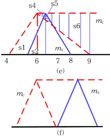
4 6 7 8 9 mx
mc
s4 s5
s1 s2
s6
(e)
mx
mc
(f)
Fig 3.2 Various type of by
For example, in [Fig 3.2] (a) and [Fig 3.2] (f), we can clearly reject the hypothesis as degree ℜ and ℜ .
For [Fig 3.2] (b), we have
ℜ
×
(3.5)
for left hand side area of center of fuzzy critical region
by fuzzy the statistics . In case of Fig 3.2 (d), we nave
ℜ
×
, (3.6)
it's maintain an uncertain attitude for decision the hypotheses.
Also, we have
ℜ
×
×
(3.6)
in Fig 3.2 (e).
4. Most powerful test of fuzzy Poisson probability
We are interested in fuzzy random variable which has fuzzy probability density function(p.d.f.) or proba- bility mass function(p.m.f) where ∈, is parameter space. We assume that ≃ or ≃
where and are fuzzy subset of .
We label the fuzzy hypothesis as
≃ versus ≃ . (4.1)
sample ⋯ from the distribution of .
A test of versus is based on a fuzzy subset
of sample space . The fuzzy set is called the fuzzy critical region and its corresponding decision de- gree rule is:
reject
by ℜ(accept by ℜ) if ⊂ (4.2) or retain
by ℜ(reject by ℜ) if ⊂. (4.3) Note that a fuzzy test is defined by fuzzy critical region. Conversely a fuzzy critical region defines a fuz- zy test.
The size of significance level of the test is denote by the probability of a type I error, i.e.,
max ≃
⊂ . (4.4) Also, the power function of a fuzzy test is given by
⊂ ≃ . (4.5) We will show the fuzzy significance level and fuzzy power function in next time.
In general, there will be a multiplicity of fuzzy sub- sets ′ of the sample space such that
⊂′ .
Suppose that there is one of these fuzzy subset , such that when is true, the power of the test associated with is greaer than the power of the test asso- ciated with each other ′. Then is defined as a best fuzzy critical region of size for testing against
.
Well known Neyman and Pearson theorem, if we have fuzzy random sample ⋯ from then the joint p.d.f. of ⋯ is
⋯ ⋯ . (4.6) Let and be distinct value of , and be a pos- itive fuzzy number. Let C to be the subset of sample space which satisfy
⋯
⋯
≺ (4.7)
for each point ⋯∈
then, in accordance with the theorem, C will be a best critical region of size for testing the fuzzy simple hypothesis.
This inequality can be can frequently expressed in form ⋯ ≺ , where is a constant. Since and are given constants,
⋯ is fuzzy statistics; and if the p.d.f. of this statistics can be found when is true, then the significance level of fuzzy test of .
Let denote fuzzy random samples from a distribution which has a pmf of Poisson distribution.
If we have probability and
per unit interval by any random experi- ment for level then we have mean
and for time
.
It is desired to test the fuzzy hypothesis
≃ against the alternative simple hypothesis
≃ . Here,
⋯
⋯
(4.8)
≺ ≻ (4.9)
If ≻ , from the set of points we have
ln ≺ ln (4.10)since ln
≺ ,
≻
ln
ln
(4.11)
is a best fuzzy critical region . Consider the case of
and , we have the best fuzzy critical region .
If we have random samples
, ,
,
then , the reject degree is ℜ
by [Fig 3.2] (b).
The case of data then reject degree is ℜ as [Fig 3.2] (d).
Finally, if we have then reject de- gree is ℜ by [Fig 3.2] (e).
References
[1] P. X. Gizegorzewski, Testing Hypotheses with vague data, Fuzzy Sets and Systems. 112 , pp.501-510, 2000.
[2] M. K. Kang, G. T. Choi and C. E. Lee, On Statistical Test for Fuzzy Hypotheses with Fuzzy Data, Proceeding of Korea Fuzzy Logic and Intelligent System Society Fall Conference, Vol.
10, Num. 2, 2000.
[3] M. K. Kang, G. T. Choi and S. I .Han, A Bayesian Fuzzy Hypotheses testing with Loss Function, Proceeding of Korea Fuzzy Logic and Intelligent Systems Society Fall Conference, Vol 13, Num. 2, 2002.
[4] M. K. Kang, C. E. Lee and S. I. Han, Fuzzy Hypotheses Testing for Hybrid Numbers by Agreement Index, Far East Journal of Theoretical Statistics, 10(1), 2003.
[5] M. K. Kang, Y. R. Park, Fuzzy Binomial Proportion Test by Agreement Index, Journal of Korean Institute of Intelligent Systems, Vol 19, Num. 1, 2009.
[6] W. Trutschnig, A strong consistency result for fuzzy relative frequencies interpreted as estimator for the fuzzy-value probability, Fuzzy Sets and Systems, 159, pp 259-269, 2008.
[7] Z. Xia, Fuzzy Probability System: fuzzy proba- bility space(1), Fuzzy Sets and Systems, 120, pp.469-486, 2001.
저 자 소 개
강만기(Man Ki Kang)
한국지능시스템학회 논문지 Vol.15 No.2, Vol.17, No.5 참조
서현아(Hyun A Seo)
현재 : 동의대학교 대학원 정보통계학과 박사과정
관심분야 : 퍼지데이터처리
![Fig 3.1 Acceptance and rejection region For various kinds of , we can reject the hypotheses by Definition 3.2 as [Fig 3.2]](https://thumb-ap.123doks.com/thumbv2/123dokinfo/5452605.435327/3.892.86.431.130.310/acceptance-rejection-region-various-kinds-reject-hypotheses-definition.webp)