Fault Diagnosis Method based on Feature Residual Values for Industrial Rotor Machines

(1)

Manuscript received July 3, 2018, Accepted November 12, 2018

1 KEPCO Research Institute, Korea Electric Power Corporation, 105 Munji‐Ro Yusung‐Gu, Daejeon 34056, Korea

2 Seoul National University, Department of Mechanical and Aeropsace Engineering, 1 Gwanak‐ro, Gwanak‐gu, Seoul, Korea

This paper is licensed under a Creative Commons Attribution‐NonCommercial‐NoDerivatives 4.0 International Public License. To view a copy of this license,

Fault Diagnosis Method based on Feature Residual Values for Industrial Rotor Machines

Donghwan Kim

^1†

, Younhwan Kim

¹

, Joon‐Ha Jung

²

, Seokman Sohn

¹

Abstract

Downtime and malfunction of industrial rotor machines represents a crucial cost burden and productivity loss. Fault diagnosis of this equipment has recently been carried out to detect their fault(s) and cause(s) by using fault classification methods. However, these methods are of limited use in detecting rotor faults because of their hypersensitivity to unexpected and different equipment conditions individually. These limitations tend to affect the accuracy of fault classification since fault‐

related features calculated from vibration signal are moved to other regions or changed. To improve the limited diagnosis accuracy of existing methods, we propose a new approach for fault diagnosis of rotor machines based on the model generated by supervised learning. Our work is based on feature residual values from vibration signals as fault indices. Our diagnostic model is a robust and flexible process that, once learned from historical data only one time, allows it to apply to different target systems without optimization of algorithms. The performance of the proposed method was evaluated by comparing its results with conventional methods for fault diagnosis of rotor machines. The experimental results show that the proposed method can be used to achieve better fault diagnosis, even when applied to systems with different normal‐state signals, scales, and structures, without tuning or the use of a complementary algorithm. The effectiveness of the method was assessed by simulation using various rotor machine models.

Keywords: Fault Detection, Feature Residual Values, Steam Turbine Diagnosis, Power Plant

I. INTRODUCTION

Rotor machines, such as steam/gas turbines, pumps, fans, and compressors, typically consist of complex mechanical systems. Such machines are essential parts of power plants and are usually designed to operate for 24 hours a day. A breakdown thus implies interrupted electricity supply, with the possibility of enormous economic losses.

Indeed, many rotor machines experience catastrophic failure due to system faults such as unbalance, misalignment of rigid and flexible couplings, shaft cracking, rubbing, and rotor bending [1]. If ignored, such faults may result in heavy financial losses and even endanger life. The accurate detection of malfunctions and the application of appropriate remedial measures are thus of the utmost importance.

To ensure early detection of abnormalities and avoid potential damage, automatic detection of faults is highly desirable from an application point of view, and this has motivated several relevant developmental studies. Because potential faults are more difficult to detect, the development

of fault diagnosis and prognosis technologies for rotor machines have attracted considerable research interest over the past few years. Various fault diagnosis systems have been developed for rotor machines, such as physical model‐based [2][3] and data‐driven fault diagnosis methods [4]‐[7]. The performance of model‐based methods is outstanding if an accurate physical model of the system is obtained [8].

However, owing to the difficulty of developing a precise mathematical model of a rotor machine, fault detection techniques that do not require a model have attracted great attention. This has created an incentive to solve most fault diagnosis problems using data‐driven methods. From a data‐

driven approach perspective, fault diagnosis is an essentially

supervised fault classification problem and can thus be cast

in a statistical pattern recognition framework [9]. The basic

idea behind classification is to find an objective function f(x)

which decides predetermined fault class y, to each training

data; the data are collected from failed condition of the

system [10]. In this regard, there is a broad range of the

strategies and technologies of the ongoing development. For

(2)

example, Sheng‐Fa Yuan et al. (2006) conducted fault detection on a rotor using a support vector machine (SVM) technique known as the “one to others” algorithm [11][12].

Combinations of statistical pattern classifiers and feature extraction techniques, such as principal component analysis (PCA) [13], kernel principal component analysis (KPCA) [14], partial least squares (PLS) [15], and independent component analysis (ICA), have also been proposed [16]. Qiang Zhao (2013) proposed a method for early diagnosis of fault in a rotor machine using a combination of PCA and a fuzzy C‐

means algorithm [17]. Fisher discriminant analysis (FDA) has also been used for fault diagnosis of rotor machines by a reliability and environmental engineering group [18].

Unfortunately, many existing methods based on supervised learning can only be applied to a rotor machine with consistent properties. In reality, the normal region of the vibration signal depends on each individual operating environment. It depends on the machine’s inherent feature differences, maintenance history and initial defects. For this reason, the normal regions of the signal obtained from equal machines may be different and the regions are changed during operation. In case of supervised fault classification methods, it works efficiently for trained and similar signatures only. The methods generate erroneous results when encounters novel data not belonging in the domain of training data [19]. In order to use the methods to correctly classify new data, the supplement steps are also needed, either generalizing methods or carrying out fine‐tuning process. In the formal case, it is hard to accommodate new data such as time history of classified data for the target equipment. Also, this process requires a great deal of time and costs. In the latter case, even though it reduces classification error, the method performance is restricted in certain equipment. To alleviate this rigidness in the trained

classifier diagnostic method, there is few groups that is studying practical fault diagnosis methods at present [20].

To overcome the drawbacks of the existing methods, we propose a flexible and robust fault diagnosis method based on supervised classification. The present method utilizes a Residual Pattern Classification (RPC) algorithm based on feature residual values. The main contribution is that it may be effective to find more robust attributes (features) that can classify the particular fault. Also, the features are less affected by system operating environment mentioned above.

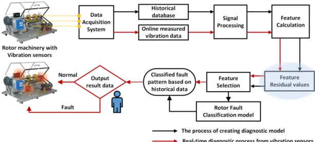
Therefore, it is possible to improve sensitivity to each fault class and accuracy of classification. Fig. 1 shows a flowchart of the RPC fault diagnosis system. The strong advantage of the method is that it generates row misclassification rate regardless of using novel data not belonging in the domain of training data. The proposed method is particularly efficient in dealing with fault diagnosis based on supervised learning.

Most of the experimental results have demonstrated its enhanced feasibility and effectiveness to industrial application compared to existing methods.

The remainder of this paper is organized as follows. In Section 2, the proposed RPC algorithm for fault diagnosis of rotor machines is presented, and the steps for implementing the algorithm are described. Section 3 describes experiments in which the existing method and the proposed method were employed in fault classification using normal‐ and fault‐state data. Results of the experiments are presented and discussed in Section 4. Conclusions drawn from the results are presented in Section 5.

II. PROPOSED ALGORITHM

In data‐driven based fault diagnosis, conventional

Fig. 1. Fault diagnosis framework of rotor machinery based on feature residual values classification approach.

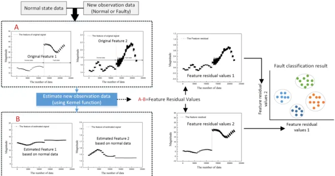
Fig. 2. Schematic of the procedure for generating the feature residual values.

(3)

methods are still used to detect some of the problems of the system, but they do not function well in the case of irregular variation of the normal‐state signal or when the system is used under different circumstances from those for which it was originally designed (see Supporting Information S1). As mentioned above, the vibration amplitude of rotor machines changes slightly over operating time. This problem is caused by inherent elements of the system, such as poor manufacturing precision of installed components and rotating shafts. Second, installed parts are usually removed and send out for a complete repair, and then the units are back in operation.

Compared to previous signals, the vibration level is changed due to some variation in position and reinstallation of the components after the repair. Third, the data obtained from identical models may not be the same because rotor machine’s design, manufacture and installing condition should naturally be different. For this reason, the accuracy of fault diagnosis only works efficiently within the operational range fixed by training data. We therefore adopted an RPC based classifier that is based on the properties of feature residual values and is not affected by uncertain parameters but can distinguish and classify normal and fault signals. The framework of the algorithm used to classify faults based on the output signal of a rotor machine is shown in Fig. 2.

The scheme for fault diagnosis by the RPC method consists of the following three steps: (1) Data matrix of vibration signal features, which are calculated from normal and faulty signal, is generated by using training data. (2) Based on auto‐associative kernel regression (AAKR), training feature‐residuals are calculated between the actual values

from the data matrix and normal state focused prediction. (3) The feature residuals are used to determine each fault pattern following feature selection and then the diagnostic model is created. (4) Real time feature residuals on new observations are obtained as comparison between a value estimated by the auto‐associative model and the corresponding measured signal. (5) Finally, the model made with past classified feature‐residuals determines what it does is locates the values in fault space.

III. EXPERIPENTS

A. Experimental setup and data acquisition criterion

To verify the proposed algorithm for the fault diagnosis of a rotor machine, data were obtained from two prototype systems and an actual system and were used to generate training and test data for fault classification and diagnostic accuracy testing. Because the vibration signal is the most powerful signal in a rotor machine and can be used to assess the condition of the machine, it was employed for the system diagnosis in this study.

Many single‐type faults (e.g., unbalance, shaft rubbing, shaft cracking, shaft bending, and misalignment) were experimentally implemented. The malfunctions were simulated using the Bently rotor kit RK4, and a prototype of a small‐

scale steam turbine and a real steam turbine system (operated in an industrial area) were used to acquire data on the fault state (see Table 1). The RK‐4 system setup (see Fig. 3(a‐1)) included a single shaft and one rotor disk with two bearings (type RK‐1) and two shafts, and one or two rotor disks (type RK‐2 and 3). The shaft had a diameter of 10 mm and a length of 500 mm. The rotor wheel had a mass of 500 g and a diameter of 80 mm. Shaft rub on the rotor system was simulated using a rub screw to make contact with the radial surface of the shaft. An unbalanced state was induced by inserting a screw with a mass of 5 g into a hole in the wheel.

The screw constituted an unbalanced mass. A crack fault was simulated by cutting a transverse slot into the shaft of the RK‐

Table 1. Explanations of training and testing data sets for each state of the rotor machine.

Test Model 1 Test Model 2

Training Data set

 Model Type: A, 1S1D

 Data number: 3,600

 Normal state: a‐1

 Model Type: B, 2S3D

 Normal state: b‐1 Test

Data set

 Normal state: a‐2

 Normal state: b‐2

Training Data set

 Data number: 3,600 Test

Data set

 Data number: 3600

Training Data set

Data set  Model Type: A, 2S2D

 Data number: 3,600  Model Type: B, 2S3D

Test Model 7 a: rotor kit

b: small‐scale steam turbine c: utility steam turbine s: shaft

d: disk Training

Data set  Model Type: A, 2S1D

Data set  Model Type: C

* a‐1: vibration level≤ 5 μm a‐2: vibration level≤10 μm b‐1: vibration level≤ 5 μm b‐2: vibration level≤10 μm b‐3: vibration level≤ 5 μm

Fig. 3. First experimental setup: (a‐1) RK‐4 rotor kit with (a‐2) displacement sensor and (a‐3) acceleration sensor, the fault imbedding device for (a‐4) mass unbalance, (a‐5) disk rubbing, (a‐6) misalignment and (a‐7) oil whirl.

Second experimental setup: (b‐1) small‐scale steam turbine prototype with (b‐2) measurement equipment, (b‐3) bearing and two shafts, the fault imbedding device for (b‐4) mass unbalance, (b‐5) disk rubbing, (b‐6) shaft rubbing, and (b‐7) misalignment. Third experimental setup: (c‐1) industrial steam turbine with (c‐2) shaft and blades and (c‐3) a bearing.

(4)

4 rotor. The crack depth was nearly one quarter of the diameter of the shaft. Misalignment was produced by the shafts of the coupled systems being mismatched relative to the centreline (see Fig. 3(a‐4 to 7)).

For the small‐scale steam turbine as shown in Fig. 3(b‐

1), the system consisted of two shafts and three rotor disks, and different fault states (mass unbalance, misalignment, and rubbing) were induced. The experimental unbalanced state was identical with that of the rotor kit, and the misalignment and rubbing fault states were induced by designing the device as shown in Fig. 3(b‐4 to 7). Vibration data for the utility steam turbine were also obtained from past events (see Fig.

3(c‐1)). All the fault and normal states were implemented at a speed of 3600 rpm since it is very important to ensure high reliability and safety of the system during its operation.

Displacement sensors were attached to the rotor machine and used to measure the distance between the sensor and the target, thereby acquire the vibration data for the horizontal and vertical orientations of the system. The measurement signals from the displacement sensors were received by an ADRE 408 DSPI data acquisition system. The raw data were then transmitted to and stored in a computer by analog‐to‐digital conversion and thereafter analyzed using MATLAB. The training/test data for the normal and fault conditions of the system were generated and used for fault classification.

B. Feature calculation from vibration sensors

After collecting useful data (i.e., information about the normal and fault states) from the target physical systems, the main features were calculated, selected, and compiled to form a feature vector that was used for training by a classification method. The calculation of the features from the vibration signal is a vital process in the fault diagnosis of a rotor machine. Because vibration signal measurement and analysis are used to generate substantial information about any fault in the machine, the features of the signal directly affect the accuracy of fault classification and detection. In this study, various statistical parameters were used to obtain the feature data in the time and frequency domains. For instance, the mean, skewness, root mean square (RMS), kurtosis, crest factor, entropy error, and lower and upper histogram bounds were applied to the time domain, whereas the frequency center (FC), root variance frequency (RVF), and RMS frequency were applied to the frequency domain (see Supporting Information S2).

C. Generation of Feature Residual values and Selection The results of the proposed RPC based fault detection method were compared with those of the general pattern recognition method. The major difference between the two methods is the addition of the step for calculating the feature residual vector in the proposed method by substituting the features obtained from the actual current (fault‐free or fault‐

induced) data for the estimated current data using historical data and AAKR function. We used the basic concepts of AAKR to estimate the measured and new observation data.

The process is based on the multivariate inferential kernel regression approach derived by Wand and Jones

(2005) [21]. In this study, historical normal‐state vibration data used to develop diagnostic model were represented by the matrix N, where N

^i,j

is the i

^th

observation of the j

^th

variables, which gives an indication of various features. For N

m,f

, m normal‐state observations and f variables, the data matrix becomes the following Eq. (1):

, ,

⋯ ,

, ,

⋯ ,

⋮ ⋮ ⋱ ⋮

,

_,

⋯

_,

(1)

In addition, using the same format, the feature value of the measured (which may be a normal or fault state) was represented by the X

1,f

, matrix X:

,

, ⋯ ,

,

(2)

As measured data was formed as Eq. (2), it was compared to each of normal‐state data matrix row to determine how similar the measured data was to each of the historical normal‐state observations. This similarity was quantified by calculating Euclidean distance between measured data and the historical normal‐state data by using Eq. (3):

,

, , , , , ,

(3)

1,2, ⋯ , , 1,2, ⋯ , This process was repeated for each of the m historical normal‐state observations, resulting in the generation of an m  1 matrix of the distance k:

, ,

⋮

,

(4)

The k matrix was then used to define weights by kernel function, as shown in Eq. (5). In this step, it is necessary to determine in advance the kernel parameter h and a type of kernel function. We therefore defined two variables to compute the estimated value of the measured data based on historical normal‐state data. Specifically, in the case of a kernel function type, there are many types of kernel functions, such as linear kernels, polynomial kernels, and Gaussian kernels. Compared with other kernel functions, the Gaussian kernel could yield the highest fault classification result in our procedure. Therefore, the Gaussian kernel was used.

1 √2 (5)

In the final step, the estimated values (E) were calculated

by combining Eq. (5) and the historical normal‐state data

matrix (N), as expressed by Eq. (6).

(5)

∑

_,

∑ (7)

We were able to obtain 3,600 sets of feature values for each condition (normal and fault states). After calculating the various feature values of the vibration signal, 32 representative features, denoted by f {f

1

, f

2

, f

3

, …, f

n

}, where n is the type of feature, were developed for each measured data of rotor system. After estimating the measured data by the above procedure, feature residual values (R) were then generated as the difference between the actual measured data and corresponding estimated values by using Eq. (7):

, , , ⋯ , , , , ⋯ ,

, , , ⋯ , (8)

where is estimated values and is feature residual values, cl is a fault class, and i = 1, 2, 3, …, n is the number of features calculated from the vibration signals. These residuals were used with important parameters to determine diagnostic model of target system. Once the feature residual values have been obtained, they were used as input data for fault classification. Table 2 gives the example of values calculated by each process.

D. Feature Selection

The features calculated from the vibration signals may still contain some irrelevant and redundant information. The classification results typically exhibit accuracy deterioration, and the handling of issue constitutes a heavy computational burden and requires huge storage space [22]. The problem is solved by feature selection to reduce the number of features and thereby improve the diagnostic accuracy. Briefly, the feature selection in this study was conducted by sorting the total saparability scores. We applied a statistical measure (t‐

test) on each feature residuals and compared total p‐value as a measure of how sensitive it was at separating groups. After that, each a feature residual value was ranked by total saparability scores using following Eq. (8).

Var / var /

. .

(8)

where st is the number of rotor status, v and q indicate types of rotor status and n is the number of data points used in variation.

We selected the top ranked 5 features, G {R

a

, R

b

, R

c

, R

d

, R

e

}, where a, b, c, d and e denote the feature variables. The top plot in Fig. 4(a to d) shows time domain vibration signal from different states obtained from training data while the lower plots are the corresponding feature residual between measured value and predicted value based on normal condition. The Fig. 4 indicates that some feature residuals are not separable, that is, the p‐value calculated from t‐test is low and the value is eliminated from feature residual candidates.

In contrast, other feature residuals shows distinct residual

shapes and these can be used as representative feature residuals.

E. Feature residual values fault classification by using a supervised classifier

In the detection of faults in a rotor machine using the RPC based method, it is necessary to learn the patterns from the training data while the system operates under various conditions. This process is referred to as machine learning.

Pattern recognition is conducted by establishing a boundary among the training data clusters and deciding which part of the boundary the test data are applied to. In this case, FDA, SVM, Naïve and KNN with feature residual values were used to define the criteria for distinguishing between the normal and fault states. The final class membership degrees are determined by the learning process. Lastly, when one of the feature residual values ( ) of new observation data under a particular condition was entered, the Euclidean distances (between the central point of classes (P

^t

) and new observation data) were obtained by using

‖ ‖ (9)

The results obtained from Eq. (9) can then be compared to determine the region that is closest to the new observation data. Finally, the fault types with the smallest Euclidean distances D

ⁱ

can be selected as the state of the data.

Table 2. Calculation sample data obtained from vibration sensors: each table includes fault data (left), estimated values of measured data (center)

and the feature residual values obtained by RPC based algorithm (right).

The abnormal measured data (unbalance state) at fault condition

1 2 3 32

No. 1 No. 2 No. 3 No. 4 No. 5

 No. 3,600

22.33 22.31 22.79 22.22 22.88

 22.56

22.47 22.47 22.47 22.47 22.47

 22.47

0.21 0.21 0.21 0.21 0.21

 0.21

0.04 0.04 0.04 0.04 0.04

 0.04

Estimated value of measured data (unbalance state) based on normal condition

1 2 3 32

No. 1 No. 2 No. 3 No. 4 No. 5

 No. 3,600

15.68 15.72 15.74 15.67 15.74

 15.72

15.12 15.12 15.12 15.12 15.12

 15.12

0.29 0.30 0.30 0.29 0.30

 0.30

0.20 0.20 0.20 0.20 0.20

 0.20

Feature residual values at abnormal measured data (unbalance state)

1 2 3 32

No. 1 No. 2 No. 3 No. 4 No. 5

 No. 3,600

6.64 6.58 7.05 6.55 7.13

 6.83

7.34 7.34 7.34 7.34 7.34

 7.34

‐0.08



‐0.08

‐0.07

‐0.08

‐0.07

‐0.08



‐0.08

(6)

IV. EXPERIMENTAL RESULTS

To investigate the improvement of fault classification accuracy by RPC‐based method, the proposed method was evaluated, and its classification results were compared with those of the general fault classification methods. To do this, we sorted all the normal and fault data for each condition set and various classifiers classification were performed by FDA, SVM, Naïve and KNN for fault classification. The important part of the experiments is that we applied to two different conditions of the each system. We first compared the results obtained with the RPC based algorithm and the common

method in the case of normal‐state fluctuation of the target system. We then compared the fault detection reliabilities of the two methods for different target systems (i.e., the training data were obtained from one system and the test data from another system). Three rotor models were used for the validation, namely, a utility steam turbine, an RK‐4 model, and a small‐scale steam turbine prototype. The experimental data were organized by randomly but equally splitting a set of data into training data and testing data.

To obtain the training data for classifying the status of new observation , the following different experimental setups were employed: (1) RK‐4, one shaft, and one disk; (2) RK‐4, two shafts, and one disk; (3) RK‐4, two shafts, and two disks;

(4) small‐scale steam turbine prototype, two shafts, and three disks; and (5) real steam turbine system. Five fault types were simulated using the first setup (RK4, one shaft, and one disk), namely, unbalance, shaft rubbing, shaft bowing, shaft cracking, and misalignment. The training/test data were obtained from the system by changing the normal state for each fault. Next, unbalance, seal/disk rubbing, and parallel/angular misalignment were implemented for the second setup (RK4, two shafts, and one disk).

For the small‐scale steam turbine prototype, the training/test data were obtained by inducing unbalance,

(a)

(b)

(C)

(d)

(e) (f)

(g) (h)

Fig. 4. Original vibration signal (time‐domain) in four conditions and their corresponding various feature residual trends. (a) normal‐state, (b) misalignment, (c) rub, (d) crack, (e) 1s average of skewness (good case), (f) 1s deviation of crest factor (good case), (g) 1s average of max value (good case), (h) 1s deviation of shape factor (bad case).

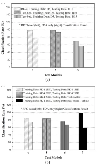
(a)

(b)

Fig. 5. Comparisons of fault identification accuracy rates of RPC based classifier and common FDA classifier for different experimental cases: the classification results obtained using (a) different baselines for the normal state and (b) identical training data and different target systems.

(7)

parallel/angular misalignment, and seal/disk rubbing under varying normal states. Finally, one set of data were obtained for the real steam turbine in the normal state and under mass unbalance and rubbing. In this experiment, the number of fault class were varied for the different systems because it was very difficult to induce or reproduce identical fault types, given the different scales and structures of the systems.

Therefore, different numbers of fault class were used to obtain the historical data and develop the classification criteria. The results of the fault classification were expressed in terms of the classification accuracies determined from Eq.

(10), where T

ⁱ

and T

ⁱⁱ

are the true fault class and the class determined by the diagnosis algorithm for the i

^th

sample, respectively.

1 If , 1, otherwise 0 (10)

Table 3 and Fig. 5 show the fault classification results obtained by, FDA, SVM, Naïve, and KNN classifiers with feature residuals. High classification accuracy was achieved with the proposed method approximately 20–25% higher than the rates achieved with the original classifiers with raw

feature values. The experimental result shown in Fig. 5 indicates that traditional fault classification methods have poor and unstable fault classification results when they encounter novel data not belonging in the domain of training data. In the other hand, the proposed method was able to distinguish between fault states and the normal‐state, despite using training and test data obtained from different normal‐

state and target systems. The maximum classification rates of the results were 99% for experiments No. 1, 2, and 7. This reflects the robustness of the RPC based algorithm for pattern recognition in a rotor machine. As expected, the RPC based diagnostic procedure can keep fault decision nicety and ignore tuning process of the algorithm even though each system has unique conditions. This means that our method itself functions as personalization, which indicate regularly interacting with the algorithm and data it is collecting. In fact, the main difference between the algorithm of the proposed method and general algorithms is the part in which the feature residual values are generated in the former for supervised fault classification. Since a lot of different conditions of the state can be appear in dynamic rotor system, some feature are invariable with phase changes (from the normal state to the fault state), whereas others may vary dramatically with changes in the main specific frequency of the system. However, when we use bare features from measured vibration signal, many important features are ignored and removed frequently during feature selection process. The reason is that the bare features from the data containing random and systematic errors result in no effect to distinguish each fault class. In the other hand, selectively sensitive feature to faults can be showed up by using feature residual values because noise reduction and disturbance suppression of feature values are occurred simultaneously during generating feature residual values between measured data and estimated data based on normal state values as shown in Fig. 6. Furthermore, if a feature value calculated from measured data is equivalent to the feature value with

Fig. 6. The example process of generating feature residual values on real data set from vibration sensors. (include normal and faulty vibration data).

Table 3. Fault diagnosis results under various classifiers with feature residuals and raw feature values. (The test are conducted by representative

experiments from No.2, 4, 5 and 7) Types of

classification

Normal state

change System change

Test Model 2 4 5 7

RPC with FDA 99% 88% 82% 99%

FDA Only 82% 75% 82 60

RPC with SVM 83 76 80 90

SVM only 59 70 72 76

RPC with Naı̈ve 85 99 98 100

Naı̈ve only 57 50 82 56

RPC with KNN 91 87 89 98

KNN only 81 75 86 65

(8)

corresponding historical normal‐state database, the difference between the estimated and measured data converges to zero, resulting in effective fault classification. In contrast, the other features, which are strongly influenced by changes in the system state, have more distinguishable features residual values than those of zero‐value feature residual values.

Accordingly, feature residual values such as {R

1cl

, R

2cl

, …, R

ncl

} provide valuable information for feature selection and fault classification. However, the RPC based classification algorithm is incapable of distinguishing all possible fault classes from the normal‐state in certain cases. The fault model does not guarantee outstanding reliable fault diagnosis result due to its intrinsic nature. The experimental results, such as experiment No. 4 and 6 (See Fig. 5), show that the classification accuracies have declined, and some fault class was observed to overlap. The accuracy results for these two cases were 85% and 76%, respectively. From this viewpoint, our diagnostic process have a tendency to take low accuracy when the model applies to system with normal‐

state fluctuation as old system has, compared to other system with different operating condition. To minimize the inconsistency of fault detection, our algorithm uses error weighting factor in feature residual values before training process is conducted.

Applying extra weights to the feature residual values of the training data reduces the differences between the training data obtained from one system and the testing data obtained from new observations of the system with different operating condition. This additional step permits adjustment to match the specific characteristics of the vibration signal from the two systems: something that originally cannot be the same, given their scales, structures, and environmental discrepancies. Furthermore, the modification not only enables the maintenance of the trend and character of the training data for fault classification in the case of identical classes but also allows for a wide margin that enables application to the case of different fault classes (see Supporting Information S3). Fig. 7 show the fault

classification accuracies achieved by adding weighting factor process to proposed diagnostic method. It can be observed that the application of the weighting factor to the training data improved the fault classification accuracy as much as 99%

in the cases of experiments 4 and 6 (see Fig. 7(d) and (f)). The technique has the advantage of not requiring a change of the datum point to distinguish between the normal and fault states. It is also suitable for the system to obtain the training data for supervised learning process. However, the proposed method requires further study to optimize the detection of other faults that were not considered in the present study, to increase the true detection rate, regardless of occurring unknown changes in the target system, and achieve a robust diagnostic ability that is applicable to any system.

V. CONCLUSIONS

In this paper, industrially high acceptable and robust fault diagnosis method were developed by using feature‐

residual values based on vibration signal and supervised classification algorithms. The weakness of the existing methods could be alleviated by feature‐residual values.

Several sets of vibration features in the time and frequency domain are calculated from the data obtained from rotor machines. The residual values are then provided by reconstructing of current vibration signal features under historical data collected during normal condition. Finally, fault classification is accomplished. The performance of the proposed method was demonstrated by using different types of data, especially including industrial steam turbine data.

Although supplemental procedures, such as fin‐tuning of the algorithm and obtaining labeled data again for supervised learning, were not conducted, the application of the method has shown that it provided a more accurate and robust classification results than traditional fault diagnosis methods.

Thus, the proposed method is a good alternative to applying identical algorithm to many similar systems without modification. We believe that our developed fault diagnosis

(a) (b) (c) (d)

(e) (f) (g)

Fig. 7. Visualization of the classification obtained by the RPC based diagnosis algorithm by changing the normal state of the system using four selected features.

(9)

method could be very effective without a man on duty. Also, it could be great potential for offering a solution to perform commercial fault diagnosis of steam turbines in power plants.

ACKNOWLEDGEMENT

This study was supported by the Power Generation &

Electricity Delivery of the Korea Institute of Energy Technology Evaluation and Planning (KETEP), with funding from the Ministry of Trade, Industry, & Energy.

REFERENCES

[1] Edwards, S., Lees, A., Friswell, M., "Fault diagnosis of rotating machinery." Shock and Vibration Digest, 30, (1), 1998, 4‐13.

[2] Jalan, A. K., Mohanty, A. R., "Model based fault diagnosis of a rotor–bearing system for misalignment and unbalance under steady‐state condition." J. Sound Vibr., 327, (3‐5), 2009, 604‐

622. [3] Sekhar, A. S., "Crack identification in a rotor system: a model‐

based approach." J. Sound Vibr., 270, (4‐5), 2004, 887‐902.

[4] Mahadevan, S., Shah, S., "In Plant Wide Fault Identification using One‐class Support Vector Machines." Fault Detection, Supervision and Safety of Technical Processes, 2009, pp 1013‐

1018.

[5] Li, C. J., Shin, H., "In Tracking Bearing Spall Severity Through Inverse Modeling." ASME 2004 International Mechanical Engineering Congress and Exposition, Anaheim, California, USA, 2004, pp 49‐54.

[6] Juričić, Đ., Moseler, O., Rakar, A., "Model‐based condition monitoring of an actuator system driven by a brushless DC motor. Control Engineering Practice." (5), 2009, 545‐554.

[7] Angelov, P., Giglio, V., Guardiola, C., Lughofer, E., Luján, J. M.,

"An approach to model‐based fault detection in industrial measurement systems with application to engine test benches." Measurement Science and Technology, 17, (7), 2006, 1809.

[9] de Araujo Ribeiro, R. L., Jacobina, C. B., Cabral da Silva, E. R., Lima, A. M. N., "Fault detection of open‐switch damage in voltage‐fed PWM motor drive systems." Power Electronics, IEEE Transactions, 18, (2), 2003, 587‐593.

[10] Yang, Q., "Model‐based and data driven fault diagnosis

methods with applications to process monitoring." Case Western Reserve University, 2004.

[11] Piramanrique, M., Francisco, R., Sofrony Esmeral, J., "Data driven fault detection and isolation: a wind turbine scenario."

Tecnura, 19, (44), 2015, 71‐82.

[12] Yuan, S.‐F., Chu, F.‐L., "Support vector machines‐based fault diagnosis for turbo‐pump rotor." Mechanical Systems and Signal Processing, 20, (4), 2006, 939‐952.

[13] Santos, P., Villa, L., Reñones, A., Bustillo, A., Maudes, J., "An SVM‐Based Solution for Fault Detection in Wind Turbines."

Sensors, 15, (3), 2015, 5627.

[14] Allgood, G. O., Upadhyaya, B. R., "In Model‐based high‐

frequency matched filter arcing diagnostic system based on principal component analysis (PCA) clustering." AeroSense International Society for Optics and Photonics, 2000, pp 430‐

440. [15] Li, P., Li, X. J., Jiang, L. L., Yang, D. L., "Fault Diagnosis for Motor Rotor Based on KPCA‐SVM." applied mechanics and materials, 2011, 143‐144, 680‐684.

[16] Li, Y., Wang, Z., Yuan, J., "On‐line Fault Detection Using SVM‐

based Dynamic MPLS for Batch Processes." Chinese Journal of Chemical Engineering, 14, (6), 2006, 754‐758.

[17] Zhu, H. Q., Fang, R. M., Peng, C. Q., "The Application of ICA‐SVM Method for Identifying Multiple Faults in Asynchronous Motors." Applied Mechanics and Materials, 483, 2013, 405‐

408. [18] Zhao, Q., "The Study on Rotating Machinery Early Fault Diagnosis based on Principal Component Analysis and Fuzzy C‐means Algorithm." Journal of Software, 8, (3), 2013, 709‐715.

[19] Tao, X., Lu, C., Lu, C., Wang, Z., "An approach to performance assessment and fault diagnosis for rotating machinery equipment." EURASIP J. Adv. Signal Process, (1), 2013, 1‐16.

[20] Ma, J., Jiang, J., "Applications of fault detection and diagnosis methods in nuclear power plants: A review." Progress in Nuclear Energy, 53, (3), 2011, 255‐266.

[21] Yin, S., Wang, G., Karimi, H. R., "Data‐driven design of robust fault detection system for wind turbines." Mechatronics 24, (4), 2014, 298‐306.

[22] Technical Review of On‐line Monitoring Techniques for Performance Assessment. Vol. 3.

[23] Liu, Z., Zuo, M. J., Xu, H., "Feature ranking for support vector machine classification and its application to machinery fault diagnosis." Proceedings of the Institution of Mechanical Engineers, Part C: Journal of Mechanical Engineering Science 2012, 2077‐2089.

(10)

Supporting Information

Supplementary Section 1. Effect of changes in the rotating system to normal signal of vibration

Fault diagnosis based on data driven methods depends on measured data (normal and fault data) and the fault classification accuracy is seriously affected by the data. For example, the diagnostic model created by using RK4 1S1D system (the data is used as training data) is hard to be applied to diagnosis of small steam turbine prototype without modifying the diagnostic model. The reason is that the criteria of diagnostic model varies according to normal state of training data. Fig. S1 shows that one rotating system has different vibration signal property from the other rotating system.

Supplementary Section 2. Various features used in making rotating diagnostic model

To properly make a diagnostic model of rotating machine, a set of features from time and frequency domain is used (see Table S1). The feature can be any signature or characteristic derived from sensor data. In this paper, we used 32 features for the detection of specific fault modes. In case of time‐domain features, each parameter was calculated from three different types of criteria such as mean per cycle, one sec average and one sec deviation of vibration amplitudes.

(a)

(b)

(c)

(d)

Fig. S1. Analysis of normal state vibration signal via different rotating systems. Time‐domain, frequency‐domain plots and Standard normal distribution of vibration signal from different rotating systems such as (a) RK4 1S1D System, (b) RK4 2S1D System, (c) Small steam turbine prototype, (d) Real Steam Turbine (S: Shaft, D: Disk).

Table S1. Description of feature parameters used in machine learning for fault classification

Signal Position Feature parameters

Time domain Frequency domain

Vibration Vertical

Horizontal Mean Skewness RMS Shape factor Kurtosis Crest factor Impulse factor Max value Entropy

Frequency center Root variance frequency Root mean square frequency 1×/2×

1×/(Total‐1×)

(11)

Supplementary Section 3. Improvement method to increase and maintain fault classification rate

(a)

(b)

Fig. S2. (a) The application of effective weighting factor used to increase and maintain fault classification rate for rotor machines, (b) the example graph of feature residual values obtained by differentiating the weighting factor.