Allocation of Energy Storage Capacity for Large Wind Farms in Korea using Discrete Fourier Transform

Manuscript received March 28, 2016, revised August 2, 2016, accepted August 18, 2016

Allocation of Energy Storage Capacity for Large Wind Farms in Korea using Discrete Fourier Transform

Seung-pil Moon†, Remund Labios, Byung-hoon Chang, Soo-yeol Kim, Yong-beum Yoon

KEPCO Research Institute, Korea Electric Power Corporation, 105 Munji-ro, Yuseong-gu, Daejeon 34056, Republic of Korea

† [email protected]

Abstract

In 2013, a total capacity of 591.3 MW of installed wind power generation was achieved in Korea, with a total of 1,139 MWh of wind energy generated that year. More wind power plants will be installed in the coming years, and it is important to develop methods to reduce the output variability of these resources so as to provide stable power to the power grid of Korea. In this regard, this paper proposes the use of energy storage system (ESS) as a means to stabilize the output variability of wind power plants. Presented in this paper is a method that uses Discrete Fourier Transform (DFT) to determine the ESS capacity needed to provide a stable power output for ancillary services such as frequency regulation, economic dispatch, and emergency reserves. In the first step of the proposed method, four regions (namely, Samdal, Yeongdeok, Yeongyang, and Gangwon) in Korea that had the most wind power generation capacity were selected for analysis. In the second step, the individual and aggregated wind power outputs of the selected regions in 2013 were obtained This information was then used in the third step, where DFT analysis of the power outputs was used to drive the magnitudes of the output variation. And finally, the ESS capacity requirements needed to provide different ancillary services were determined based on the magnitudes of the output variation.

Keywords: Energy storage, energy storage system, discrete Fourier transformation, wind energy

I. INTRODUCTION

As stated in the “6th Basic Plan for Long-Term Electricity Supply and Demand (BPE)” released by the Ministry of Trade, Industry and Energy of Korea, 17 GW of wind power capacity will have to be installed by 2027 [1]. As of October 31, 2015, the total generating capacity stood at approximately 805 MW with expansion efforts currently underway to meet the 2027 goal. As an example, among the on-going expansion projects is the construction of a 2.5 GW offshore wind farm located at the southwest coast of Korea [2]. Due to the amount of planning and construction that still needs to be done to reach a capacity of 17 GW, the development of a method to determine the best locations to install wind farms is necessary.

Using wind as a renewable energy resource to provide power to the Korean grid poses a challenge in maintaining secure and stable power due to the variability of the output produced by wind turbines. The issue of output variability thus requires the development of necessary technologies and methodologies that will minimize output variability and allow existing power systems to accommodate more renewable energy power plants.

One strategy for reducing the variability of wind power is by aggregating wind farms that cover a large geographical area.

The aggregation of wind farms creates a smoothing effect:

individual wind farms with different wind utilization rates are grouped into a synthesized system, thereby producing a single output with minimal variability compared to each generation unit or wind farm alone [3][4]. Another strategy for mitigating the variability of wind power is by using energy storage systems (ESSs), which can be used in the power system in a variety of forms (e.g., CAES, electrochemical batteries, and flow batteries)

to provide a variety of services (e.g., renewable power output smoothing, peak shaving, and frequency regulation). Also, the studies show that ESS can improve the operational reliability of wind power systems and aid in the reduction of electricity production costs [5]-[8].

Reference [9] presents an approach in using DFT as a tool to determine the optimal size of energy storage required for a power system with a high penetration of renewable energy. After obtaining the the wind power output signal that represents the energy storage output, the wind power output signal is then decomposed into time-varying components that represent the existing operational protocols of a power system. These components can be categorized as intra-week, intra-day, intra- hour, and real-time.

To take advantage of the combined benefits gained from using aggregated wind farms and ESS, this paper proposes an approach to determine the size of the ESS capacities that will be integrated with wind farms to provide ancillary services, such as frequency regulation, standby operating reserves, 1-hr emergency reserves, and load shifting. This study used SCADA output data that encompassed 10 days during the period of March 10-19, 2014 from four wind farms in Korea. The wind output data was then decomposed into time-varying components using Discrete Fourier Transform (DFT) analysis. The time periods used in this study reflect the current operational protocols being used in the Korean power grid: 0-5 min for frequency regulation, 5-20 min for standby operating reserves, 20 min to 1 hr for one- hour emergency reserve service, 1-2 hr for alternative reserves, and 1-6 hr for load shifting.

Section II discusses the wind farm output data used in the

study, and the fluctuation analysis that was performed. Section

III discusses the DFT process used in the study. Section IV discusses the results of the wind farm output fluctuation analysis, as well as the results obtained after performing DFT analysis on the wind farm output data. Finally, Section V presents the conclusion of the study and the authors’ recommendations for further study.

II. ANALYSIS OF WIND FARM OUTPUT DATA A. Selection of Wind Farms

This study was conducted using SCADA data with a 5- second output measurement interval obtained from March 10 to March 19 in 2014, for a total of ten days. By that time, there were 48 wind farm locations in Korea with a total generator capacity of 591 MW. The wind farms had a generation capacity ranging from 250 kW to 98,000 kW. Fig. 1 shows the annual total wind power capacity and energy output until 2014.

Four wind power plant locations out of the 48 were selected for this study. First is the Yeongdeok power plant, which is located in Yeongdeok, North Gyeongsang Province and has a generation capacity of 39,600 kW produced by 24 wind turbines.

Second is the Gangwon power plant, which is located in Pyeongchang County, Gangwon Province and has a generation capacity of 98,000 kW produced by 49 wind turbines. Third is the Yeongyang power plant, which is located in Yeongyang, North Gyeongsang Province and has a generation capacity of 61,500 kW produced by 41 wind turbines. Last is the Samdal power plant, which is located in Seogwipo City, Jeju Province and has a generation capacity of 33,000 kW produced by 11 wind turbines.

B. Analysis of Wind Output Fluctuations

Analyzing wind output fluctuations helps in determining the variations in the output, where a high amount of fluctuation means that there is a high degree of volatility with the amount of power that a wind power plant generates. The amount of fluctuation should be minimized, as a stable power output is preferable over an unstable one.

Using the 10-day SCADA data of the four selected wind farm locations, the output fluctuations at each location were calculated using the following general equation:

max (1)

In Eq. 1, R

is the amount of power fluctuation in MW, RU

is the largest ramp-up amount in MW, and RD

is the largest ramp-down amount in MW, and j is the number of data points. It should be noted, however, that although this method of data analysis is convenient for use, it does not accurately represent output variations that occur in real-time.

As shown in Fig. 2, a sliding window with a predetermined period was used in the analysis of the signal. In this study, the output signals were studied first with a 1-minute window, and then with a 5-minute window.

Based on the general equation shown in Eq. 1, the following equation was used to calculate the amount of output fluctuation in MW:

max min , ∀ 1,2, ⋯ , ⁄

if at max at min (2) if at max at min

where, i = 1,2,…,T/n j = 1,2,…,(nd - T/n)

T : period (e.g., 1 min. or 5 min.) n : sampling time

The fluctuation rate is calculated as follows:

,

100% (3)

where P

is the fluctuation rate of the output power, and P

is the generation capacity.

III. DFT ANALYSIS OF WIND OUTPUT SIGNALS A. DFT and IDFT Equations

Based on the methods presented in [3], wind power outputs were analyzed using DFT to obtain the periodic wind power output fluctuations. The general form of the DFT equation is as follows:

Fig. 1. Wind power generation in Korea (1999-2014) [10].

0 200 400 600 800 1000 1200 1400

0 100 200 300 400 500 600 700

until 1999 2000 2001 2002 2003 2004 2005 2006 2007 2008 2009 2010 2011 2012 2013 2014 Energy Output (GWh)

Power Output (MW)

Year

Energy Generated (GWh) Newly Installed (MW) Subtotal Installed (MW) Fig. 2. Illustration of the fluctuation analysis wherein a sliding window is used.

k=0,1,…,N-1 (4) The resulting DFT signal is then synthesized using the

following inverse DFT (IDFT) signal:

1

n=0,1,…,N-1 (5) In both Eq. 3 and 4, N is the number of the data points taken

along the output signal.

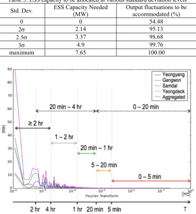
The wind power output signals were decomposed into five categories: 0-5 min for frequency regulation, 5-20 min for standby operating reserve, 20 min to 1 hr for 1-hr emergency reserve, 1-2 hr for alternate reserves, and 2-6 hr for load shifting.

Table 1 shows the specifications of these components.

Table 1. Frequency Bands and Time Periods for DFT Analysis Service or Operation f

(Hz)

f

(Hz) 1/f

1/f

Freq. Regulation 0 3.33E-03 - 5 min.

Standby Operating Reserves

3.33E-03 8.33E-04 5 min. 20 min.

1-hr Emergency

Reserves 8.33E-04 2.78E-04 20 min. 1 hr.

Alternate Reserves 2.78E-04 1.38E-04 1 hr. 2 hr.

Load Shifting 1.38E-04 4.63E-05 2 hr. 6 hr.

Fig. 3. Wind output generation (MW) and amount of output fluctuation (MW) during a 5-minute period obtained from Yeongdeok region’s wind data (March 10-19, 2014).

Fig. 4. Wind output of wind farms on March 10-19, 2014.

Fig. 5. Fluctuation rates of individual and aggregated wind farms on March 10- 19, 2014.

Fig. 6. Wind output fluctuation range for T=5 min. at the Yeongdeok region on March 10-19, 2014.

Fig. 7. Probability distribution of wind output fluctuations for T=5 min. at the Yeongdeok region on March 10-19, 2014.

0%

10%

20%

30%

40%

50%

60%

70%

Yeongyang Gangwon Samdal Yeongdeok Aggregated

Fluctuation Rate

Location

Fluctuation Rate per Minute Fluctuation Rate per 5 min.

B. Probability Density Analysis and Sizing of ESS Capacity Analysis of the probability density of the output fluctuations was done after obtaining the DFT results. The probability density analysis was done to determine the maximum output fluctuation during the 10-day period on March 10-19, 2014 to be able to determine the required size of the power and energy capacities of the energy storage system.

IV. RESULTS A. Wind Power Output Fluctuation Rates

Shown in Fig. 3 is the wind output generation in MW on March 10-19, 2014 at the Yeongdeok region, as well as the amount of output fluctuation calculated using (2) at T=5 min.

Shown in the following chart in Fig. 4 are the wind power outputs of each of the four power plants, as well as their aggregated output, during the same period in March 2014. These two figures show the variation in wind output throughout the ten-day period, and how each region differs from one another in the amount of wind power that can be generated.

The fluctuation rates of the all five outputs (four power plants and the synthesized output) summarized in Fig. 5 show that the fluctuation rate is lower in larger wind farms that have a higher number of wind turbines. It can also be seen in the figure that treating all four wind power plants as one aggregate wind farm results to a fluctuation rate that is the least among the five outputs.

Fig. 6 shows a sample of the fluctuation range for when T=5 min. taken from the wind output at the Yeongdeok region, and its probability distribution is shown in Fig. 7. The probability distribution is important for determining the ESS capacity that should be allocated to be able to “cover” or accommodate the range of output fluctuations within a certain value of T. It can be seen from Fig. 7 that the maximum and minimum limits of the fluctuation occur at a much lower probability compared to output values between, for example, -3 MW and 3 MW. From this, it may be seen that it can be impractical to allocate an amount of energy storage capacity that accommodates the maximum and minimum limits. Due to this, it was assumed in this paper that standard deviations of 2, 2.5, and 3 (instead of the maximum deviation) would be sufficient in determining the amount of energy storage to be allocated. This is further explained in Subsection IV.C.

B. DFT and IDFT Results

After analyzing the wind power output fluctuation rates at

each wind farm location and as an aggregated wind farm, DFT was then applied to the wind output signals. Shown in Fig. 8 are the DFT signals derived from the individual and aggregated power outputs of the wind farms. Each DFT signal was then transformed into IDFT signals using the time periods shown in Table 1.

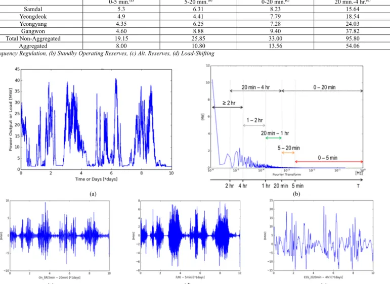
Fig. 9 shows the sample results of DFT and IDFT output transformations of the wind output signal produced by the aggregated wind farms. The wind output signal, shown in Fig.

9(a), of the aggregated wind farms is transformed in to a DFT signal in Fig. 9(b). This is then broken down into the IDFT components. Sample results are shown as follows: 5-20 min for standby operating reserves as shown in Fig. 9(c); 0-5 min for frequency regulation as shown in Fig. 9(d); and 20 min - 4 hr for reserve operations as shown in Fig. 9(e).

C. Output Probability Density Analysis and ESS Capacity Sizing After obtaining the DFT and IDFT outputs, the output probability density is analysis for each and aggregated wind farm with a capacity of 232.1 MW.

Shown in Table 2 is a sample set of results obtained for frequency regulation services having the period of 0-5 minutes.

Negative values pertain to the amount of energy or power to be absorbed by the ESS from the wind farm, while positive values pertain to the amount of energy or power to be delivered by the ESS to the grid. From this table, it can be seen that the power requirements for an aggregated wind farm (-31.3 MW, 26.7 MW) are lower than the total power requirements when wind farms are not aggregated (-43.5 MW, 36.9 MW). The lower power is a result of the smoothing effect caused by aggregating the wind farms. This lower power requirement is beneficial, as this will require ESS with a lower power capacity to provide the same amount of energy.

Table 2. Min. and max. ESS requirements, and standard deviation values occuring between the period 0-5 min for frequency regulation

Location

Wind Farm Capacity

(MW)

Energy (MWh)

Power (MW) 2.0

(MW) 2.5

(MW) 3.0

Neg. Pos. Neg. Pos. (MW)

Non- Aggregated

A 33.0 -0.34 0.44 -13.8 8.4 2.12 3.18 5.30 B 39.6 -0.43 0.43 -8.0 7.8 2.14 3.37 4.90 C 61.5 -0.56 0.57 -14.2 13.3 1.63 2.72 4.35 D 98.0 -0.41 0.39 -7.5 7.4 2.30 3.16 4.60 Total 232.1 -1.44 1.53 -43.5 36.9 8.19 12.43 19.15 Aggregated 232.1 -1.45 1.54 -31.3 26.7 4.00 5.33 8.0 A: Samdal, B: Yeongdeok, C: Yeongyang, D: Gangwon.

Table 3. ESS capacity to be allocated at various standard deviation levels Std. Dev. ESS Capacity Needed

(MW)

Output fluctuations to be accommodated (%)

0 0 54.48

2 2.14 95.13

2.5 3.37 98.68

3 4.9 99.76

maximum 7.65 100.00

Fig. 8. DFT results of wind power output signals.

Evidence of reduced fluctuations due to aggregation is also shown by the lower values of output power at 2, 2.5, and 3

when the wind farms are aggregated. This further supports the need for using aggregated wind farms in order to reduce ESS size requirements.

As ESS facilities can be expensive, several options on the amount of ESS capacity to be allocated should be considered during the planning phase. One way to achieve this is by determining the power output at standard deviation levels of 2, 2.5, and 3. Table 3 shows the amount of ESS capacity that can be allocated. As shown in the table, if 100% of the output fluctuations are to be accommodated, an ESS capacity of 7.65

MW will be required. However, if we are only to accommodate 99.76% (standard deviation of 3) of the output fluctuations, only 4.9 MW will be needed. A difference of 3 MW is a considerable amount if, for example, an ESS system would cost $100/kW.

The final determined values for the different ESS sizing requirements are shown in Table 4 and Table 5. It can be seen from both tables that the ESS capacity requirements increase as the period being considered for a particular ancillary service increases. It can also be observed that, between the energy storage requirements for non-aggregated wind farms and aggregated wind farms, lower energy requirements are needed for aggregated wind farms. In Table 4, the ESS capacities shown accommodate

Table 4. Summary of ESS capacities to be allocated based on min. and max. fluctuation limits

Location 0-5 min.

5-20 min.

20 min. - 1 hr.

1-2 hr.

2-6 hr.

MW MWh MW MWh MW MWh MW MWh MW MWh

Samdal 13.8 0.4 9.7 2.3 10.5 7.7 6.2 11.2 16.4 73.2

Yeongdeok 8.0 0.4 9.5 2.2 13.2 11.5 10.2 17.3 17.6 69.4

Yeongyang 14.1 0.6 10.2 2.3 11.1 8.3 16.9 33.0 28.3 154.7

Gangwon 7.5 0.4 11.5 2.8 17.8 12.3 22.4 39.2 49.7 222.5

Total Non-Aggregated 43.4 1.9 40.9 9.5 52.6 39.9 55.6 100.8 111.9 519.8

Aggregated 34.6 1.5 25.6 5.2 28.8 21.3 33.5 55.7 74.6 371.0

Difference between

Total and Aggregated 8.7 0.3 15.3 4.4 23.8 18.6 22.2 45.1 37.3 148.8 (a) Frequency Regulation, (b) Standby Operating Reserves, (c) 1-hr. Operating Reserves, (d) Alt. Reserves, (e) Load-Shifting

Table 5. Summary of required ESS capacities to be allocated based on 3 standard deviation

Location ESS Capacity (MW)

0-5 min.

5-20 min.

0-20 min.

20 min.-4 hr.

Samdal 5.3 6.31 8.23 15.64

Yeongdeok 4.9 4.41 7.79 18.54

Yeongyang 4.35 6.25 7.28 24.03

Gangwon 4.60 8.88 9.40 37.82

Total Non-Aggregated 19.15 25.85 33.00 95.80

Aggregated 8.00 10.80 13.56 54.06

(a) Frequency Regulation, (b) Standby Operating Reserves, (c) Alt. Reserves, (d) Load-Shifting

(a) (b)

(c) (d) (e)

Fig. 9. The wind power output in (a) produced by aggregated wind farms, goes through DFT processing. The DFT process creates the signal (b) that is then broken down

into components (c), (d), and (e).

100% of the output fluctuations. In Table 5, the ESS capacities (in MW) shown were obtained from a standard deviation of 3, and can be seen to be lower than those shown in the previous table.

Table 5 also shows different time periods for alternate reserve services and load shifting services. The main purpose for this is to show the capability of the method presented in this paper to evaluate various ancillary services that have different requirements across different electricity markets. The flexibility of this method can generate recommendations for various cases, thus providing power system engineers with a highly customizable tool when evaluating options during the planning and design phase for installing ESS resources.

V. CONCLUSION

This paper presents a methodology for determining the amount of energy storage capacity for four wind farm locations in Korea. Using SCADA data obtained from the power plants located in Samdal, Yeongdeok, Yeongyang, and Gangwon, the rate of wind output fluctuations was analyzed in each region, and collectively as an aggregated resource so as to take advantage of the smoothing effect. The wind power outputs were then analyzed using Discrete Fourier Transform so as to determine the energy requirements needed to provide ancillary services-such as frequency regulation, standby and emergency reserves, and load shifting-to the power grid.

Through this study, it has been determined that treating the separate four regions as one aggregate source of wind power, the amount of output fluctuation is reduced, and the amount of needed ESS capacity is similarly lower. A more stable output is beneficial for power systems operations, and a lower amount of needed ESS capacity is beneficial for investment costs.

It is recommended that additional studies be conducted using year-long data over multiple years from multiple regions around Korea so as to gain a better understanding of the output fluctuations produced by existing wind farms. Obtaining a wind profile of existing wind farms in Korea can aid in the expansion of additional power plant facilities that take advantage of wind

energy.

REFERENCES

[1] Ministry of Trade, Industry, and Economy (formerly, Ministry of Knowledge Economy). (2013). The 6th Basic Plan for Long-term Electricity Supply and Demand (2013–2027). [Online]. Available:

https://www.kpx.or.kr/english_new/down_data/market_report/The _6th.pdf.

[2] Korea Electric Power Corp. (2014). 2014 Annual Report. [Online].

Available:http://home.kepco.co.kr/kepco/cmmn/fms/FileDown.do

?atchFileId=FILE_000000021050868&fileSn=0.

[3] J. G. Slootweg and W. L. Kling, “Modeling of Large Wind Farms In Power System Simulations,” Power Engineering Society Summer Meeting, Chicago, IL, USA, 25 July 2002, pp. 503-508.

[4] M. G. Lobo and I. Sanchez, “Regional Wind Power Forecasting Based on Smoothing Techniques, with Application to the Spanish Peninsular System,” IEEE Trans. on Power Systems, vol. 27, no. 4, pp. 1990-1997, May 2012.

[5] P. Denholm, et al., (2013, May). The Value of Energy Storage for Grid Applications. NREL, Golden, CO. [Online.] Available: http://

www.nrel.gov/docs/fy13osti/ 58465.pdf.

[6] F. Diaz-Gonzalez, A. Sumper, O. Gomis-Bellmunt, and R.

Villafafila-Robles, “A Review of Energy Storage Technologies for Wind Power Applications,” Renewable and Sustainable Energy Reviews, vol. 6, no. 4, pp. 2154-2171, May 2012, pp. 105-112.

[7] M. Khalid and A. V. Savkin. “Minimization and Control of Battery Energy Storage for Wind Power Smoothing: Aggregated, Distributed and Semi-Distributed Storage,” Renewable Energy, vol.

64, pp. 105-112.

[8] M. C. Such and C. Hill, “Battery Energy Storage and Wind Energy Integrated into the Smart Grid,” Innovative Smart Grid Technologies, 2012 IEEE PES, Washington, DC, USA, 16-20 Jan.

2012, pp. 1-4.

[9] Y. V. Makarov, P. Du, M. C. W. Kintner-Meyer, C. Jin, and H. F.

Illian, “Sizing Energy Storage to Accommodate High Penetration of Variable Energy Resources,” IEEE Trans. On Sustainable Energy, vol. 3, no. 1, pp. 34-40, Jan. 2012.

[10] Korea Wind Energy Industry Association. (2015). (Wind Power Statistics and Information). [Online]. Available: http://kweia.or.kr.

[11] Seungpil Moon, Byunghoon Chang, Sooyeol Kim, Sungmin Choi,

Yongbeum Yoon,” ESS Allocation for Large Scale Wind Farm

Generation Fluctuation”, KIEE Power Engineering Society

Autumn Meeting, Nov. 2014.