Analysis of Geometric and Spatial Image Quality of KOMPSAT-3A Imagery in Comparison with KOMPSAT-3 Imagery

1. Introduction

KOMPSAT-3A is the sister spacecraft of KOMPSAT-3, using the same satellite bus and payload, launched on 25

of May in 2015. The satellite

provides panchromatic sensor with 55 cm ground sampling distance (GSD) at nadir and provides high resolution. Simultaneously, the multispectral sensor collects blue, green, red and near-infrared (NIR) bands with 2.2 m nadir resolution, respectively.

Analysis of Geometric and Spatial Image Quality of KOMPSAT-3A Imagery in Comparison

with KOMPSAT-3 Imagery

Nyamjargal Erdenebaatar, Jaein Kim and Taejung Kim

Department of Geoinformatic Engineering, Inha University

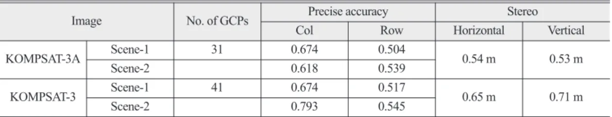
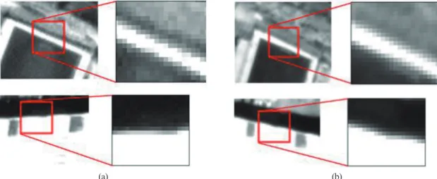
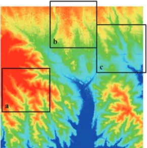
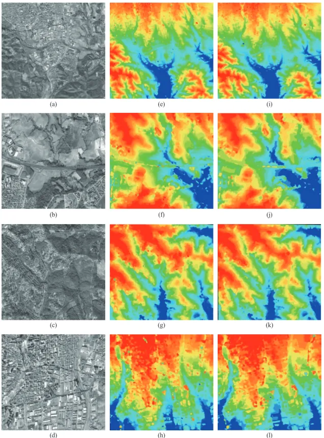
Abstract : This study investigates the geometric and spatial image quality analysis of KOMPSAT-3A stereo pair. KOMPSAT-3A is, the latest satellite of KOMPSAT family, a Korean earth observation satellite operating in optical bands. A KOMPSAT-3A stereo pair was taken on 23 November, 2015 with 0.55 m ground sampling distance over Terrassa area of Spain. The convergence angle of KOMPSAT-3A stereo pair was estimated as 58.68 ˚. The investigation was assessed through the evaluation of the geopositioning analysis, image quality estimation and the accuracy of automatic Digital Surface Model (DSM) generation and compared with those of KOMPSAT-3 stereo pair with the convergence angle of 44.80 ˚ over the same area. First, geopositioning accuracy was tested with initial rational polynomial coefficients (RPCs) and after compensating the biases of the initial RPCs by manually collected ground control points. Then, regarding image quality, relative edge response was estimated for manually selected points visible from two stereo pairs. Both of the initial and bias- compensated positioning accuracy and the quality assessment result expressed that KOMPSAT-3A images showed higher performance than those of KOMPSAT-3 images. Finally, the accuracy of DSMs generated from KOMPSAT-3A and KOMPSAT-3 stereo pairs were examined with respect to the reference LiDAR-derived DSM. The various DSMs were generated over the whole coverage of individual stereo pairs with different grid spacing and over three types of terrain; flat, mountainous and urban area. Root mean square errors of DSM from KOMPSAT-3A pair were larger than those for KOMPSAT-3. This seems due to larger convergence angle of the KOMPSAT-3A stereo pair.

Key Words : Digital Surface Model, Geometric Accuracy, Kompsat-3A, Kompsat-3

Received September 6, 2016; Revised October 26, 2016; Accepted October 27, 2016.

†

Corresponding Author: Taejung Kim ([email protected])

This is an Open-Access article distributed under the terms of the Creative Commons Attribution Non-Commercial License (http://creativecommons. org/licenses/by-nc/3.0) which permits unrestricted non-commercial use, distribution, and reproduction in any medium, provided the original work is properly cited

Article

The goal of this study is to evaluate geopositioning accuracy and analyze spatial image quality of KOMPSAT-3A imagery. The studies on the positioning accuracy and image quality assessment of high satellite imagery are significant for its further analysis, performance and applications. Regarding geopositioning accuracy evaluation, QuickBird (Noguchi et al. 2004), GeoEye-1 and WorldView-2 (Aguilar et al. 2014), Formasat-2 (Chen et al. 2006), Cartosat-1 (Baltsavias et al. 2006 and Giribabu et al.

2013) and KOMPSAT-3 (Jeong et al. 2016) images were reported. Among them, Jeong et al (2016) evaluated performance of KOMPSAT-3 stereo pair in terms of positioning and Digital Surface Model (DSM) generation and compared overall performances with those of WorldView-1 imagery. On the other hand, since newly launched satellites have mission to collect data with improved accuracy and specifications than their previous sensors, it is essential to examine performances of new satellite imagery by comparing with older satellite data regarding 3D positioning and spatial image quality. For example, the geolocation accuracy of KOMPSAT-3 stereo images was evaluated and compared with that of KOMPSAT-2 images (Jeong et al. 2014). This study demonstrated that KOMPSAT-3 showed higher location accuracy than that of KOMPSAT-2.

Due to these reasons, we aimed to analyze the geometric performance and spatial image quality of KOMPSAT-3A imagery and compare with those of KOMPSAT-3 images in this paper. The performance comparison of KOMPSAT-3A and KOMPSAT-3 stereo pair was assessed through the evaluation of the geopositioning analysis, image quality estimation and the accuracy of automatic DSM generation.

Geopositioning accuracy was tested with initial rational polynomial coefficients (RPCs) and after compensating the biases of the initial RPCs by ground control points (GCPs). GCPs were collected manually on clearly identifiable features on satellite images and a

reference DSM generated from LiDAR point clouds.

Total 41 GCPs were used for the analysis and among them 31 GCPs were included in the KOMPSAT-3A stereo coverage. Spatial image quality was analyzed by estimating relative edge response (RER) for manually selected points visible from two stereo pairs. Various DSMs were generated over the whole coverage of individual stereo pairs with different grid spacing and over three types of terrain; flat, mountainous and urban area. The results were compared to a reference DSM derived from LiDAR point clouds.

2. Study site and datasets 1) Study site

The test site is covering Terrassa area (Fig. 1) located in Catalonia region of Spain. International Society for Photogrammetry and Remote Sensing (ISPRS) Working Group I/4 (Reinartz et al. 2010) provides benchmarking data set located in Catalonia, Spain. The test field covers both of mountain and urban areas.

2) KOMPSAT-3A data

KOMPSAT-3A stereo dataset was acquired on 23 November, 2015. The processing level of satellite stereo pair was Level 1R; the images were sensor and radiometrically corrected. Each image is 24060 by 16800 pixels and presented in Fig. 2. The physical GSD

Fig. 1. Test site.

for the nadir view of KOMPSAT-3A is 0.55 m. Due to the incidence angles using in stereo model, GSD reaches up to 0.75 m. The scenes were taken with incidence angles of 36.91˚ to the left and 35.49˚ to the

right resulting in a base-to-height (B/H) ratio of 1.22 (Table 1). The stereo data set was provided with respective RPCs and metadata file. The specification of KOMPSAT-3A stereo pair is summarized in Table Fig. 2. KOMPSAT-3A (above) and KOMPSAT-3 (below) stereo images.

Table 1. The specifications of stereo pairs

KOMPSAT-3A KOMPSAT-3

Scene-1 Scene-2 Scene-1 Scene-2

Product level Level 1R Level 1R

Spectral mode PAN PAN

Orbit direction Ascending orbit Ascending orbit

Acquisition date 23-Nov-15 5-Feb-13

GSD 0.75 m 0.73 m 0.88 m 0.91 m

Incidence angle 36.91˚ 35.49˚ 30.60˚ 32.04˚

Convergence angle(base to height ratio) 58.68˚ (1.22) 44.80˚ (0.82)

Altitude 540.57 km 541.06 km 695.91 km 697.50 km

Elevation angle 53.08˚ 54.51˚ 59.40˚ 57.96˚

Azimuth angle 143.32˚ 9.79˚ 32.66˚ 126.91˚

Roll -17.06˚ -16.76˚ -18.53˚ -20.48˚

Pitch -29.24˚ 28.27˚ 19.85˚ -20.16˚

Bisector elevation angle 73.88˚ 67.50˚

Asymmetry angle 0.88˚ 1.22˚

Image size 24060×16280 24060×16800 24060×18416 24060×17832

3 and compared to KOMPSAT-3 images.

Imaging geometry of satellite stereo pair can be expressed by the parameters, convergence (α), BIE (β), and asymmetry angles (γ) (Fig. 3). The convergence angle has been defined as the angle between two rays of stereo pair; the BIE angle is the elevation angle of the bisector of the convergence angle; the asymmetry angle is measured between the bisector and the line perpendicular to the baseline (Jeong et al. 2016). These parameters were calculated by the equation introduced by Jeong et al. (2015) and used with B/H ratio for the relationship analysis to the geometry accuracy of the DSMs.

3) Ground points collection and LiDAR data Accuracy of rational polynomial coefficients (RPCs) based stereo model can be further improved by using ground control points (GCPs) (Giribabu et al. 2013).

GCPs are points identifiable in real space, whose location are known and they are used to refine the orientation of images. 41 GCPs distributed over the study were measured and selected carefully on images.

Among them, 31 points were included in the KOMPSAT-3A stereo images. The distribution of GCPs on the overlapping area is presented in Fig. 4.

Since many researchers proposed the use of highly accurate LiDAR derived DSM as ground truth to check accuracy of DSM generated from very high resolution satellite images (Aguilar et al. 2014), the LiDAR-

derived DSM was used as a reference DSM for accuracy analysis of automatic DSM generation in this study. The data set provided by ISPRS Working Group I/4 include LiDAR point clouds. It was acquired with approximately 0.3 points per square meter. Its coverage area is small region of KOMPSAT-3A images, about 6 km × 6 km with variable terrain relief (both flat and hilly) (Fig. 5).

3. METHODS

1) Bias compensated object points determination

Geo-positioning accuracy was tested with initial RPCs and after compensating the biases of the initial RPCs. A practical means of modeling and subsequently

Fig. 5. LiDAR-derived DSM.

Fig. 3. Representation of stereo geometry.

Fig. 4. Distribution of GCPs in the coverage of datasets and

examples.

compensating for the biases inherent in RPCs is through a block-adjustment approach introduced by Grodecki and Dial (2003). The model equations are defined in Equation (1).

r

= c

=

(1) P

(X

, Y

, Z

) = a

+ a

X

+ a

Y

+ a

Z

+ a

X

Y

+ a

X

Z

+ a

Z

X

+ a

X

+ a

Y

+ a

Z

+ a

X

Y

Z

+ a

X

+ a

Y

X

+ a

Z

X

+ a

X

Y

+ a

Y

+ a

Z

Y

+ a

X

Z

+ a

Y

Z

+ a

Z

where (r

, c

) are the normalized row and column on the image space; (X

, Y

, Z

) are the normalized longitude, latitude, and ellipsoidal height of their corresponding ground coordinates on the object space.

Parameters a

, a

…, a

are the coefficients of the polynomial function P

and the coefficients of P

, P

and P

are defined similarly. The model coefficients were extracted from the RPCs provided by vender (Jeong et al. 2015). Forty one model GCPs were used to compensate for the errors in the model coefficients and then the model equations were precisely updated.

The error compensation in the image space was estimated by Equation (2).

∆p = a

+ a

*Column + a

*Row (2) ∆r = b

+ b

*Column + b

*Row

where ∆p and ∆r are the adjustable functions in the column and row directions respectively, and a

, a

, a

, b

, b

, b

are the image adjustment parameters that can

be estimated by a least-square adjustment.

Fig. 6. illustrates the procedure of rational function model (RFM) bias compensation. Starting from the object space, the 3D object coordinates (X, Y, Z) are mapped to RFM coordinates (x’, y’) by using RPCs.

2) Image quality analysis

There are various ways of describing image quality.

From engineering side, GSD, modulation transfer function (MTF), signal-to-noise ratio (SNR), relative edge response (RER) and so on (Kim and Kim. 2011).

The one part of this study is to evaluate accuracy of automatic DSM generation based on image matching algorithm. Since image matching depends on image quality, evaluating image quality is also key concern to analyze quality of DSM generated from KOMPSAT- 3A images.

In this experiment, we used RER estimation method proposed previously (Choi and Helder, 2005; Kim and Kim, 2011) and estimated RER value of KOMPSAT- 3A and compared with that of KOMPSAT-3 stereo pair. In this method, initial edge points are selected and edge profile is extracted after determining edge orientation. Then point spread function is generated.

3) Automated DSM generation

Developed matching algorithm is based on grey- level correlation on pixels applied along epipolar lines.

P

(X

,Y

,Z

) P

(X

,Y

,Z

) P

(X

,Y

,Z

) P

(X

,Y

,Z

)

Fig. 6. The procedure of RFM bias compensation. Fig. 7. Edge response curve.

Accurately matched points were extracted by applying grey level correlation windows and selecting best candidates by relaxation. And by using multiple correlation windows, more accurate image matching than the existing area based matching technique is possible. In addition, by using the pyramid-based technique the matching stability was enhanced. Once stereo image matching was completed for all matching pairs, a DSM from each pair was extracted (Rhee and Kim, 2015). The patch sizes were set to 15×15 and 23×23 pixels for this experiment.

As a mentioned above, the convergence angle can be defined as the angle between two rays that intersect at a common ground point, one from the fore image and one from aft image, measured along the convergence or epipolar plane. In addition, the base-to-height ratio is defined by the separation of the pair derived by the height of the sensor. Theoretically, an angle between 30˚ to 60˚ would be ideal whereas a base-to-height ratio between 0.5 and 1.0 is usually the most appropriate for

DSM creation (Aguilar et al. 2014).

4. EXPERIMENT RESULT

1) Analysis of geopositioning accuracy Geo-positioning accuracy was tested with initial RPCs and after compensating the biases of the initial RPCs provided with images. For accuracy check, 41 GCPs which are clearly identifiable features were examined and selected very carefully. Among them, 31 GCPs were included on the coverage of KOMPSAT- 3A stereo pair. Table 2 summarizes initial positioning errors of KOMPSAT-3A stereo pairs and compared with that of KOMPSAT-3 images.

The estimation expressed that initial positioning accuracy of KOMPSAT-3A stereo pair are quite smaller than those of KOMPSAT-3 pair. Then, the direction and magnitude of initial positioning errors in the image space of KOMPSAT-3A and KOMPSAT-3

Fig. 8. Initial positioning errors of KOMPSAT-3A images. (a) Scene-1 and (b) Scene-2.

(a) (b)

Table 2. Initial geo-positioning accuracy of KOMPSAT-3A and KOMPSAT-3 images

Image No. of GCPs Initial accuracy Stereo

Col Row Horizontal Vertical

KOMPSAT-3A Scene-1 Scene-2 31 13.67 18.40 2.83 2.03 10.55 m 9.94 m

KOMPSAT-3 Scene-1 Scene-2 41 46.10 26.50 9.12 4.09 26.62 m 14.63 m

images are presented in Fig. 8 and Fig. 9, respectively.

Then, positioning accuracy of KOMPSAT-3A and KOMPSAT-3 images was evaluated after compensating

the biases of initial RPCs. The updated geo-positioning accuracy using GCPs is shown Table 3. The magnitude and direction of errors are illustrated in Fig. 10 and Fig.

Fig. 10. Updated positioning errors of KOMPSAT-3A images. (a) Scene-1 and (b) Scene-2.

(a) (b)

Fig. 11. Updated positioning errors of KOMPSAT-3 images. (a) Scene-1 and (b) Scene-2.

(a) (b)

Fig. 9. Initial positioning errors of KOMPSAT-3 images. (a) Scene-1 and (b) Scene-2.

(a) (b)

11, respectively.

Same as the initial positioning accuracy, that the precise errors of KOMPSAT-3A stereo pair were evaluated as sub-meter; 0.54 m in horizontal and 0.53 m in vertical. This result presents that positioing accuracy of KOMPSAT-3A was higher compsare to KOMPSAT-3 images inspite of fewer number of GCPs used for analysis.

2) Estimaton of RER

Image quality analysis was examined for KOMPSAT-3A and KOMPSAT-3 stereo pairs by estimating RER. The points visible from two stereo pairs were selected manually on both of the image pairs. For the examination, 121 edge points were extracted from the five targets. The distributions of these points are presented in Fig. 12 regarding Scene- 1 of two satellites.

Therefore, MTF compensation analysis was performed for the stereo pairs using these extracted points. Table 4 presents the results of MTF analysis and demonstrates that MTF compensation has not been applied to both of stereo images.

Three enlarged examples of above five locations are presented in Fig. 13 and the extracted edge points are illustrated by red lines. Fig. 14 shows comparison of same edges on the two stereo image pairs. Estimated RER values are summarized in Table 5 regarding each scene of two satellites.

Table 5 expresses that edge response of KOMPSAT- Table 3. Updated geo-positioning accuracy of KOMPSAT-3A and KOMPSAT-3 images

Image No. of GCPs Precise accuracy Stereo

Col Row Horizontal Vertical

KOMPSAT-3A Scene-1 Scene-2 31 0.674 0.618 0.504 0.539 0.54 m 0.53 m

KOMPSAT-3 Scene-1 Scene-2 41 0.674 0.793 0.517 0.545 0.65 m 0.71 m

Fig. 12. Distributions of extracted edge points (a) over Scene-1 of KOMPSAT-3A and (b) Scene-2 of KOMPSAT-3.

(a) (b)

Table 4. MTF compensation analysis of KOMPSAT-3A and KOMPSAT-3 images

Scene-1 Scene-2

KOMPSAT-3A 6.18 % 5.93%

KOMPSAT-3 4.11 % 3.19%

3A images is higher than that of KOMPSAT-3 stereo pair regarding each scene. This is due to the different GSD estimated from stereo pairs. In terms of scenes, the RER value estimated from Scene-1 (GSD = 0.75

m) of KOMPSAT-3A is smaller than that of Scene-2 (GSD = 0.73m) , whereas the edge response of Scene-2 (GSD = 0.91 m) of KOMPSAT-3 is lower in comparison with Scene-1 (GSD = 0.88 m).

The example of edge response function is illustrated in Fig. 15. According to the curve and examined RER results, KOMPSAT-3A pair showed higher edge resposnse and has imporved image quality.

Fig. 15. Edge response profile of KOMPSAT-3A and KOMPSAT-3 images.

Fig. 13. The example of extracted egde points (illustrated by red lines) from Scene-1 of KOMPSAT-3A image.

Fig. 14. Comparison between enlarged edges for (a) KOMPSAT-3A and (b) KOMPSAT-3.

(a) (b)

Table 5. RER values of KOMPSAT-3A and KOMPSAT-3

Scene-1 Scene-2

KOMPSAT-3A 0.4240 0.4323

KOMPSAT-3 0.3986 0.3804

3) DSM generation and quality analysis Automatic DSMs with various grid spacing of 1 m, 2 m and 5 m were generated from KOMPSAT-3A stereo pair. DSMs were examined over the whole coverage of individual stereo pairs and three types of terrain; flat, mountainous and urban area. The comparison areas are presented in Fig. 16 and generated DSMs at 2 m grid spacing from KOMPSAT-

3A and KOMPSAT-3 images are compared in Fig. 17.

Even though there is not totally flat area in the reference DSM, the most appropriate region was selected as flat in this study.

Root Mean Square (RMS) Errors of generated DSMs were estimated over these areas and whole coverage area with respect to the reference LiDAR point clouds. Table 6 summarized the accuracy comparison of generated DSMs from KOMPSAT-3A and KOMPSAT-3 over the same area. Overall, the quality of the extracted DSMs largely depended on the target land cover, being better for DSMs covering flat areas than those attained over urban areas or the entire working area.

Visual analysis demonstrates that DSMs from KOMPSAT-3A have showed lower performance than those from KOMPSAT-3. For instance, a whole coverage DSM (Fig. 17.e) from KOMPSAT-3A has more blunders in the center region compare to DSM from KOMPSAT-3. If we see comparison terrains of flat, mountainous and urban areas in detail, differences are quite clear. Due to DSM extraction is dependent from terrain; the errors in flat area are relatively smaller than other comparison areas. In contrast, derived DSM over urban area presents observable differences.

Fig. 16. Coverage of three comparison terrain by overlapping LiDAR DSM. (a) Mountainous area, (b) urban area and (c) flat area.

Table 6. DSM quality results of KOMPSAT-3A and KOMPSAT-3

DSM Grid spacing Image type Flat area Mountainous Urban Whole area

KOMPSAT-3A

1.0 m Patch 15 4.0568 6.5275 6.0819 5.1876

Patch 23 4.1715 7.0221 6.4117 5.1905

2.0 m Patch 15 4.1355 6.2865 6.0636 5.3436

Patch 23 4.4319 6.9968 7.6458 5.2178

5.0 m Patch 15 4.4753 6.7509 6.2686 5.5120

Patch 23 4.4031 7.1472 6.7358 5.4857

KOMPSAT-3

1.0 m Patch 15 3.6753 5.5064 5.1843 4.4982

Patch 23 3.5597 5.4069 5.1461 4.6449

2.0 m Patch 15 3.8354 5.5868 5.5009 4.6300

Patch 23 3.7209 5.6603 5.4878 4.7432

5.0 m Patch 15 4.2317 6.3391 6.0434 5.2201

Patch 23 4.2764 6.6609 6.0600 5.2948

Fig. 17. Visual analysis spatial image (Scene-1 of KOMPSAT-3A) and generated DSMs from KOMPSAT-3A (e-h) and KOMPSAT-3 (i-l) with 2 m grid spacing in case of whole coverage (a, e, i), flat (b, f, j), mountainous (c, g, k) and urban area (d, h, l), respectively.

(d) (h) (l)

(a) (e) (i)

(k) (g)

(c)

(b) (f) (j)

In terms of effect of the correlation window size on automated DSM generation, RMSEs show interesting results. For example, accuracies of most DSMs derived from KOMPSAT-3A stereo pair are higher when patch size is equal to 15. Regarding KOMPSAT-3 images, more than half extracted DSMs and especially, all whole area DSMs have lower RMSEs when patch size is selected as 15. Moreover, since DSM with 1 m grid spacing has highest quality, calculated RMSEs of both of whole area DSMs with 1 m are smaller if patch size is 15.

In theory, satellite imaging geometry, generally B/H ratio or convergence angle, influences extensively in the improvement of DSM accuracy.

Thereby, we concluded that due to wider convergence angle and larger B/H ratio (α=58.68˚ and B/H=1.22) of KOMPSAT-3A stereo pair, stereo geometry parameters have adversely affected to the DSM quality.

5. CONCLUSION

In this study, the geometric performance and spatial image quality of KOMPSAT-3A stereo pair was examined. The geometric accuracy of KOMPSAT-3A stereo was assessed through the evaluation of the geopositioning analysis, image quality estimation and the accuracy of automatic DSM generation. The satellite image pair was processed as Level 1R products with GSD of 73 cm and 75 cm. Overall performances were compared with analyses KOMPSAT-3 images with GSD of 88 cm and 91 cm taken over the same area. Geo-positioning performances of the initial and after compensating the biases were demonstrated that 3D position of KOMPSAT-3A showed higher accuracy than those of KOMPSAT-3 images. Then, image quality assessment result expressed that KOMPSAT-3A stereo pairs showed better relative edge response compare to KOMPSAT-3 images in case of each scene. Eventually, the accuracy of DSMs

over whole coverage and three types of terrain; flat, mountainous and urban area, generated from KOMPSAT-3A and KOMPSAT-3 stereo pairs were examined with respect to the reference DSM. RMSEs of DSM from KOMPSAT-3A pair were larger than those for KOMPSAT-3. Theoretically, convergence angle between 30˚ to 60˚ would be ideal whereas a B/H ratio between 0.5 and 1.0 is usually the most appropriate for DSM creation. In this study, both of convergence angle and base-to-height ratio of KOMPSAT-3A stereo pair are higher compare to KOMPSAT-3 images and we concluded that these parameters have achieved lower performance of DSM generation.

References

Aguilar, M.Á., M. Saldaña, and F.J. Aguilar, 2014.

Generation and quality assessment of Stereo- Extracted DSM from Geo-Eye-1 and WorldView-2 imagery, IEEE Transaction of Geoscience and Remote Sensing, 52(2): 1259- 1271.

Baltsavias, E., S. Kocaman, and K. Wolff, 2008.

Analysis of Cartosat-1 images regarding image quality, 3D point measurement and DSM generation, The Photogrammetric Record, 23(123): 305-322.

Chen, L.C., T.A. Teo, and C.L. Liu, 2006. The geometrical comparisons of RSM and RFM for FORMASAT-2 satellite images, Photogrammetric Engineering & Remote Sensing. 72(5): 573-580.

Choi, T and D. Helder, 2005. Generic sensor modeling

for modulation transfer function (MTF)

estimation, Proc. of 2005 ASPRS Pecora 16-

Gloval Priorities in Land Remote Sensing,

South Dakota, USA, Oct 23-27, Digitally

available on CD.

Grodecki, J. and G. Dial, 2003. Block adjustment of high-resolution satellite images described by rational polynomials, Photogrammetric Engineering & Remote Sensing, 69: 59-68.

Giribabu, D., P. Kumar, J. Mathew, K.P. Sharma, and Y.V.N.K. Murthy, 2013. DEM generation using Cartosat-1 stereo data: issues and complexities in Himalayan terrain, European Journal of Remote Sensing, 46: 431-443.

Jeong, J., J. Kim, and T. Kim, 2014. Analysis of geolocation accuracy of KOMPSAT-3 imagery, Korean Journal of Remote Sensing, 30(1): 37- 45.

Jeong, J., C. Yang, and T. Kim, 2015. Geo-positioning accuracy using multiple-satellite images:

IKONOS, QuickBird, and KOMPSAT-2 stereo images, Remote Sensing, 7: 4549-4564.

Jeong, J., C. Yang, and T. Kim, 2016. Quantitative estimation and validation of the effects of the convergence, bisector elevation, and asymmetry angles on the positioning accuracies of satellite stereo pairs, Photogrammetric Engineering &

Remote Sensing, 82(8): 625-633.

Jeong, J., J. Kim, T. Kim, and S. Rhee, 2016. Evaluation of the performance of KOMPSAT-3 stereo

images in terms of positioning and the generation of digital surface models, Remote Sensing Letters, 7(10): 955-964.

Kim, T. and J. Kim, 2011. Automated assessment of NIIRS and GRD of high resolution satellite images through edge profile analysis of natural targets, Proc. of JACIE 2011 Civil Commerial Imagery Evaluation Workshop, Digitally available on CD.

Kim, T. and S. Rhee, 2015. Automated DSM extraction from UAV images and performance analysis, The International Archives of the Photogrammetry, Remote Sensing and Spatial Information Sciences, 40(1): 351.

Noguchi, M., C.S. Fraser, T. Nakamura, T. Shimono, and S. Oki, 2004. Accuracy assessment of Quick Bird stereo imagery, The Photogrammetric Record, 19(106): 128-137.

Reinartz, P., P. D’Angelo, T. Kraub, D. Poli, K.

Jacobsen, and G. Büyüksalih, 2010.

Benchmarking and quality analysis of DEM

generated from high and very high resolution

optical stereo satellite data, The International

Archives of Photogrammetry and Remote

Sensing, 38(1): 1-6.