ISSN 1225-0988 | EISSN 2234-6457 <Original Research Paper>
Identification of DEA Determinant Input-Output Variables : an Illustration for Evaluating the Efficiency of
Government-Sponsored R&D Projects
Sungmin Park †
Department of Business Administration, Baekseok University
DEA 효율성을 결정하는 입력-출력변수 식별 : 정부지원 R&D 과제 효율성 평가를 위한 실례
박 성 민 백석대학교 경상학부
In this study, determinant input-output variables are identified for calculating Data Envelopment Analysis (DEA) efficiency scores relating to evaluating the efficiency of government-sponsored research and develop- ment (R&D) projects. In particular, this study proposes a systematic framework of design and analysis of experi- ments, called “all possible DEAs”, for pinpointing DEA determinant input-output variables. In addition to corre- lation analyses, two modified measures of time series analysis are developed in order to check the similarities between a DEA complete data structure (CDS) versus the rest of incomplete data structures (IDSs). In this em- pirical analysis, a few DEA determinant input-output variables are found to be associated with a typical public R&D performance evaluation logic model, especially oriented to a mid- and long-term performance perspective.
Among four variables, only two determinants are identified : “R&D manpower” ( ) and “Sales revenue” ( ).
However, it should be pointed out that the input variable “R&D funds” ( ) is insignificant for calculating DEA efficiency score even if it is a critical input for measuring efficiency of a government-sponsored R&D project from a practical point of view a priori. In this context, if practitioners’ top priority is to see the efficiency be- tween “R&D funds” ( ) and “Sales revenue” ( ), the DEA efficiency score cannot properly meet their expec- tations. Therefore, meticulous attention is required when using the DEA application for public R&D perform- ance evaluation, considering that discrepancies can occur between practitioners’ expectations and DEA effi- ciency scores.
*
Keywords: Data Envelopment Analysis, Design of Experiments and Analysis, Determinant Input-output Variables, Efficiency, R&D Performance Evaluation
1. Introduction
1.1 Motivation
The program logic model of public research and development (R&D) performance evaluation can be defined as a pictorial model that explains how a program does its work. The pro-
gram logic model links resources with planned activities and performance (Wholey, 1983; Bickman, 1987; Wholey, 1987;
McLaughlin and Jordan, 1999). W. K. Kellogg Foundation (WKKF) (2004) classifies performance according to three dif- ferent time periods : (1) short-term (1~3 years) outputs, (2) mid-term (4~6 years) outcomes and (3) long-term (7~10 years) impacts-most of which have occurred since the com-
†Corresponding author : Professor Sungmin Park, Department of Business Administration, Baekseok University, Cheonan, Korea (ROK), 330-704, Tel : +82-41-550-2497, Fax : +82-41-550-9172, E-mail : [email protected]
Received June 1, 2013; Revision Received July 22, 2013; Accepted September 2, 2013.
pletion of a program. Ruegg and Feller (2003) propose a pro- gram logic model for the performance evaluation of the Advanced Technology Program (ATP) at National Institute of Standards and Technology (NIST) under the U.S. Depart- ment of Commerce (DOC). McLaughlin and Jordan (1999) propose a flow-chart type program logic model to describe the process of “a research and technology development and deployment program” of the Office of Energy Efficiency and Renewable Energy (EERE) under the U.S. Department of Energy (DOE).
In recent years, the performance efficiency and effective- ness of public R&D investment has been analyzed using a variety of methodologies based on program logic models.
Quantitative and qualitative evaluation obtained from the for- mative as well as the summative perspective can be fed back into subsequent decisions so as to enhance the overall rele- vance and accountability of an R&D program. For example, Government Performance Results Act (GPRA) was enacted by the U.S. Congress in 1993; all government affairs have been evaluated for performance since then (GPRA, 2003).
Similarly, the Korean government also established a national R&D program performance assessment and management system in 2006; all activities and performance of each government-sponsored R&D project (i.e., GSP) is monitored yearly during the subsequent five-year performance follow- up period (MST․KISTEP 2007).
1.2 Statement of the Problem
Bitman and Sharif (2008) mention that Data Envelopment Analysis (DEA) is one of the representative methodologies for measuring R&D performance efficiency. But they point out that practitioners tend to be reluctant to use it due to its mathematical complexity. Rouse and Putterill (2003) pro- posed “an integral performance framework”; they discussed three major components: performance measurement, analysis and evaluation. Also, they selected three typical methods for the analysis of performance productivity-Stochastic Frontier Analysis (SFA), Total Factor Productivity (TFP) and DEA.
Chiesa and Masella (1996) emphasized the importance of identifying tangible performance measures as a prerequisite step for successful R&D performance evaluation. Meanwhile, this study is initiated from pondering the three biggest diffi- culties in practical use of DEA as pointed out by Seiford and Thrall (1990): (1) model specification, (2) variables’ weights (i.e., multipliers) restrictions and (3) variables selection.
First, regarding model development and selection, a variety of DEA-related literature has been reported since the CCR (Charnes, Cooper and Rhodes) model was proposed. The CCR model is based on the assumption of Constant Returns
to Scale (CRS) for the first time (Charnes et al., 1978). Then, the BCC (Banker, Charnes and Cooper) model was established with a Variable Returns to Scale (VRS) assumption, which can be regarded as a variant of the CCR model (Banker et al., 1984). Additionally, Banker and Morey (1986a) developed a DEA model that can handle exogenously fixed variables. Banker and Morey (1986b) presented a mixed-integer programming-based DEA model to deal with categorical variables. Also, Charnes et al. (1985), widened the model selection, providing a DEA/
Window Analysis (DEA/WA) model that can encompass the passage of time (i.e., dynamic) analysis. Applications of DEA- based Malmquist Index (MI) can be found, associated with analyzing R&D performance productivity changes between two points in time. Here, productivity changes are separated by two components : “catch-up” (i.e., rate of efficiency change) and “frontier-shift” (i.e., rate of technical change) (Wu et al., 2006; Guan and Chen, 2010).
Second, to date some types of DEA multiplier constraints are designed with the aim of improving the reliability of the DEA efficiency score. Typically, two types of multiplier con- straints are proposed : the Cone-Ratio (CR) model by Charnes et al. (1990) and the Assurance Region (AR) method by Thompson et al. (1990). Generally, AR multiplier constraints are classified into three subordinate types as follows : (1) ab- solute Weights Restrictions (WRs), (2) relative WRs or AR Type I (AR-I), (3) input-output WRs or AR Type II (AR-II) (Cooper et al., 2004). Furthermore, the AR Global Model (ARGM) can restrict virtual input-virtual output (Wong and Beasley, 1990; Allen et al., 1997; Pedraja-Chaparro et al., 1997). Asmild et al. (2007) also reported experimental results on the sensitivity of DEA efficiency scores associated with CR model-type multiplier constraints.
But, disappointingly, it is still not easy to find DEA-related literature with empirical analyses as well as theoretical dis- cussions explaining a systematic procedure, especially for DEA input-output variables selection, sampling of homogeneous data (i.e., outliers elimination) and so on. Particularly, due to the model’s aforementioned mathematical complexity, practitio- ners tend to doubt DEA efficiency scores. Regarding DEA in- put-output variables like this, they may ask : “Do they really work in the calculation of DEA efficiency scores in accord- ance with their own importance?” But until now, the liter- ature has not offered many clear-cut answers about that.
With this question in mind, this study aims to bridge this
gap. First, determinant input-output variables are identified
that overwhelm the other remaining insignificant variables in
DEA efficiency score calculation when evaluating the effi-
ciency of government-sponsored R&D projects. Second, it is
examined whether or not determinants match the variables that
practitioners consider relatively more important a priori. Fi-
Figure 1. R&D performance evaluation logic model(An integrated model excerpted from McLaughlin and Jordan, 1999; Ruegg and Feller, 2003; WKKF, 2004)
nally, statistical characteristics are summarized using an em- pirical analysis. In particular, the experimental design and analysis framework developed in this study with so-called
“all possible DEAs” is based on the concept of “all possible regressions”-that is, a typical regression variable selection and model building procedure. In addition to correlation analyses, two modified accuracy measures of time series analysis are developed and examined in order to check the similarities between a DEA complete data structure (CDS) versus incomplete data structures (IDSs). Section 2 of this paper provides background and theory, Section 3 provides design of experiments, Section 4 provides analysis of experi- ments and Section 5 offers practical implications and con- clusions.
2. Background and Theory
2.1 R&D Performance Evaluation and Generic Program Logic Models
<Figure 1> is a generic program logic model for public R&D performance evaluation (McLaughlin and Jordan, 1999;
Ruegg and Feller, 2003; WKKF, 2004). In particular, Ruegg and Feller (2003), illustrate some representative factors of the inputs as well as the three-phased subsequent perfor- mance in the ATP Toolkit, Part I. Inputs include budget, staff, etc. Meanwhile, some intellectual property-related outputs are listed including publications and patents. Commercializa- tion-related outcomes are new-improved products, processes
and services, firm growth, etc. For the socio-economic long-term impacts, we can see employment gains, international competi- tiveness and so on.
Lee et al. (2009), utilize a DEA/AR model in their public R&D performance efficiency study in order to consider the importance of input-output variables associated with six het- erogeneous R&D programs. Hsu and Hsueh (2009), evaluate DEA efficiency of 110 GSPs; consequently, they emphasize the need for an appropriate upper limit on the ratio of the amount of government support in the R&D budget. Bitman and Sharif (2008), compare characteristics of five common methodologies for R&D performance evaluation : (1) scoring model, (2) Analytic Hierarchy Process (AHP), (3) Boston Consulting Group (BCG) or growth-share matrix, (4) Bal- anced Scorecard (BSC) and (5) DEA. Abramo et al. (2008), reported a DEA application for bibliometric data in the Italian university system for measuring the technical effi- ciency of research activities. Sharma and Thomas (2008), compared the national R&D programs of 22 countries and found that a small number of R&D programs conducted by developing countries were benchmarks located on the DEA efficiency frontier. Meng et al. (2006), analyzed the relative efficiency of investments for some basic research programs in China using statistical regressions and DEA method. They found that there were significant improvements in overall ef- ficiency from 1991 to 1996. Oral et al. (1991), presented three R&D project evaluation and selection models : self- evaluation model, cross-evaluation model and selection model.
Farris et al. (2006), presented a case study of how DEA
was applied to compare engineering design projects of the
Belgian Armed Forces, and they explained a variablereduc- tion process where the initial 23 input-output variables were reduced to the final five input-output variables. Zhu (2003), discussed some DEA sensitivity studies regarding the varia- ble and model selection, and a regression-based model was proposed for identifying critical input performance measures related to a case with only one output variable. Treatment of data variations by statistical methods has been proposed in re- lated literature as well. Simar and Wilson (2000), used a boot- strap method which could deal with multiple input-output variables, and they proposed a general method for bootstrap- ping in nonparametric frontier models to remedy the sam- pling variations resulted from a finite sample of observed production units.
2.2 DEA Models and All Possible Regressions DEA is a methodology of Operations Research (OR) that calculates relative efficiency scores of a set of peer entities in the range of [0, 1]. Each entity pursuing the same objective that is called Decision Making Unit (DMU) has common multiple input-output variables. Initially, active fields of DEA applications are education programs (Charnes and Cooper, 1980; Charnes et al., 1981; Bessent et al., 1982), urban police department (Parks, 1983), banking center (Sherman and Gold, 1985), hospitals (Banker et al., 1986) and so forth. Moreover, Seiford and Thrall (1990), Callen (1991), Zhu (2003), Cooper et al. (2004) and Cooper et al. (2007), presented excellent ex- planations particularly on mathematical formula and compu- tational implementation for various DEA models.
Unlike typical statistical analysis methodologies (e.g., re- gression analysis) that mainly focus on the analysis of central tendency, DEA explores the extreme surface of data (i.e., frontier). Statistical analysis is used to find the relative posi- tion of the individual from the center of data, while DEA is used to measure the relative position of the individual from the frontier of data. Therefore, DEA as an extreme-point te- chnique is very sensitive to data measurement error and out- liers which can lead to a serious problem (Seiford and Thrall, 1990). From the input-oriented perspective, DEA frontier is the minimum input to achieve a given output. On the con- trary, it means the maximum output with given input from the output-oriented point of view.
Assume a set of DMUs ( , ⋯ , ) having input variables ( , ⋯ , ) and output variables( , ⋯ ,
). Then, for each , “semipositive” vectors of input- output variables are defined as ∈ × , ∈ × . For all DMUs, matrices of input-output variables are defined as
∈ × , ∈ × . Eq. (1) is a CCR ratio model that calculates DEA efficiency score
of (Zhu, 2003; Cooper et al., 2004; Cooper et al., 2007). In Eq. (1), ∈ × , ∈ × are vectors of in- put-output multipliers respectively and every element of
× ∈ × , × ∈ × has a value of zero.
subject to ≤ ∀ (1)
≥ ×
≥ ×
By applying Charnes and Cooper transformation such as (1) , (2) and (3) to Eq. (1), a non- linear fractional programming model Eq. (1) can be convert- ted into a linear programming model Eq. (2) that is a CCR multiplier model (Seiford and Thrall, 1990; Callen, 1991).
subject to ≤ × (2)
≥ ×
≥ ×
By adding VRS assumption, Eq. (2) is modified to an in- put-oriented multiplier infinitesimal VRS model Eq. (3). In Eq. (3), the decision variable is a VRS scalar. To disting- uish between “efficiency” and “weak efficiency”, constraints are also modified so that , have values greater than or equal to infinitesimal or non-Archimedean . Every element of × ∈ × , × ∈ × has a value of ε and all elements of ∈ × are ones. Hence, “the production possibility set” enveloped by the frontier is defined as Eq.
(4). In Eq. (4), ∞ ∞ cor- responds to four different Returns To Scale (RTS) assump- tions such as CRS, VRS, IRS (Increasing Returns to Scale), DRS (Decreasing Returns to Scale) respectively and a semi- positive ∈ × is a vector of DMU intensity (Cooper et al., 2007).
subject to ≤ × (3)
≥ ×
≥ ×
free in sign
∣≥ ≤ ≤ ≤ ≥ × (4)
Meanwhile, in regression analysis, a variety of computa-
tional methodologies have been developed associated with
regression variable selection, especially for building parsi-
monious models (Montgomery et al., 2001). The most
Figure 2. DEA’s complete data structure(i.e., a mid- and long-term performance oriented model of
“2012 PTDAS”)
widely used methods are : (1) all possible regressions, (2) di- rected search on t-statistic and (3) stepwise regression. Fur- thermore, the stepwise regression can be classified into three types : (1) forward selection, (2) backward elimination and (3) stepwise regression. Basically, the full model which in- cludes all regression variables acts as the reference for re- gression variable selection. By checking statistics between the full model and reduced models, statistically significant regression variables can be identified, which is the core of these methodologies. Key statistics examined are (adjusted-) coefficient of multiple determination, residual mean square, Mallows and so on.
3. Design of Experiments
3.1 DEA Data Structures for All Possible DEAs
<Figure 2> shows that the DEA data structure analyzed in this study consisted of four input-output variables of a GSP (i.e., DMU) associated with “2012 R&D Program of Tech- nology Development and Application Support (PTDAS)”, described in detail in Section 3.2. In fact, “2012 PTDAS” is one of the major R&D programs sponsored by the Ministry of Knowledge Economy (MKE) of Korea; the budget spent from 2006 to 2010 was approximately 0.6 billion U.S. dollars (MKE․NIPA, 2012). To establish the data structure, this study considered the availability of the MKE․NIPA data- base and the data reliability. As seen in a generic R&D per- formance evaluation logic model in <Figure 1>, short-term intellectual property outputs (e.g., publications, patents, etc.) should be included in the data structure along with mid-term commercialization outcomes and long-term socio-economic impacts. However, most beneficiaries of “2012 PTDAS” are small and medium-sized enterprises (SMEs) or venture busi- nesses involved in the information and communication tech- nology industry, so intellectual property outputs are not the
main interest of this study. Therefore, the data structure in
<Figure 2> can be considered as a design of limited scope, coping with the chain of “R&D funds” ( ) and “R&D man- power” ( ) → “Sales revenue” ( ) and “New employment”
( ).
In order to identify determinants in calculating DEA effi- ciency scores among four input-output variables shown in
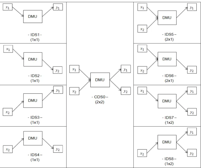
<Figure 2>, a total of nine different data structures for all possible DEAs are generated. This is shown in <Figure 3>.
In <Figure 3>, “CDS0” is the complete data structure (CDS) with (the number of inputs the number of outputs) = (2 ×2)as in <Figure 2>. Compared with “CDS0”, the other eight in- complete data structures (IDSs) are presented on both sides of the compartments in <Figure 3>. On the left-hand side, four ( × = 2×2 = 4)(1×1) IDSs are listed from “IDS1”
to “IDS4.” On the right-hand side, the upper two ( ×
= 1×2 = 2)(2×1) and the lower two ( × = 1×2 = 2)(1
×2) IDSs are arranged from “IDS5” to “IDS8.” Similar to the computational procedure of all possible regressions, “CDS0”
serves as a reference in the comparisons of data structures explained hereafter.
3.2 Data collection and Sample
<Table 1> explains the DEA input-output variables con- sidered in this study. The first input variable, “R&D funds”
( ) is the sum of two sub-items such as “Amount of government support” ( ) and “Corporate matching funds”
( ). The second input variable, “R&D manpower” ( ) is the sum of two sub-items such as “Technical manpower”
( ) and “Non-technical manpower” ( ). Meanwhile, the
first output variable, “Sales revenue” ( ) is the aggregate of
pure sales of products and services through a GSP occurring
during the five-year performance follow-up period from 2006
to 2010. The second output variable, “New employment” ( )
is also the aggregate of pure new employment in the same
manner as “Sales revenue” ( ). Two variables, “R&D man-
power” ( ) and “New employment” ( ) are collected in
the units of man-years. For measuring these two output varia-
bles, each GSP’s contribution is reflected as well.
Figure 3. DEA’s complete data structure versus incomplete data structures
DEA input variable Variable name Year of input Sub-items
R&D funds = + 2006 Amount of government support ( ) Corporate matching funds ( ) R&D manpower = + 2006 Technical manpower ( ) Non-technical manpower ( ) DEA output variable Variable name Performance follow-up period Sub-items
Sales revenue New employment
2006~2010 2006~2010 Table 1. DEA input-output variables
In “2012 PTDAS”, all activities and performance of all 796 GSPs that launched between 2006 and 2010 were inves- tigated and assessed by MKE of Korea. Among them, 218 GSPs that started and finished in 2006 provide a good sample for this study; the R&D performance time-lag can be fully reflected.
Among the initial sample, 133 companies responded to the
“2012 PTDAS” survey and submitted their GSPs-related ob- servations (response rate = 133/218×100 = 61%). Only 37 GSPs reported “Sales revenue” ( ) and “New employment”
( ) created during the five-year performance followup peri-
od (the ratio of performance creation = 37/133×100 = 28%).
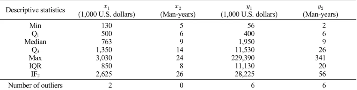
Table 2. Box-plot outliers screening for DEA data set Descriptive statistics (1,000 U.S. dollars)
(Man-years)
(1,000 U.S. dollars)
(Man-years) Min
Q 1
Median Q 3
Max IQR IF 2
130 500 763 1,350 3,030 850 2,625
5 6 9 14 24 8 26
56 1,950 400 11,530 229,390 11,130 28,225
2 6 9 341 26 20 56
Number of outliers 2 0 6 6
Table 3. DEA data set
GSP ID DMU ID (1,000 U.S. dollars)
(Man-years)
(1,000 U.S. dollars)
(Man-years) 3B-06-0008-00
3B-06-0027-00 3B-06-0058-00 3B-06-0164-00 3B-06-0192-00 3B-06-0194-00 3Z-06-0044-00 3Z-06-0054-00 3Z-06-0060-00 3Z-06-0073-00 3Z-06-0074-00 3Z-06-0078-00 3Z-06-0085-00 3Z-06-0091-00 3Z-06-0098-00 3Z-06-0111-00 3Z-06-0126-00 3Z-06-0137-00 3Z-06-0139-00 3Z-06-0158-00 3Z-06-0177-00 3Z-06-0181-00 3Z-06-0182-00 3Z-06-0206-00 3Z-06-0230-00 3Z-06-0241-00 3Z-06-0246-00 3Z-06-0262-00
1 2 3 4 5 6 7 8 9 10 11 12 13 14 15 16 17 18 19 20 21 22 23 24 25 26 27 28
2,000 445 600 523 765 564 300 200 945 2,047 959 300 249 1,161 697 997 572 509 1,975 180 500 560 763 890 1,200 150 130 764
15 6 12 9 10 6 6 5 5 24 23 6 7 23 13 8 7 6 13 5 6 8 8 6 14 5 12 5
1,950 10,000 19,300 3,828 450 300 1,600 180 428 400 56 11,416 800 384 3,167 3,280 760 1,802 340 1,464 360 2,020 100 60 4,150 690 10,409 160
6 9 19 12 14 4 36 8 2 27 7 3 2 3 24 6 6 6 10 8 8 3 2 6 9 8 12 5 StDev Mean
CoefVar Min
Median
Max IQR
748.00 534.00 130.00 0.71 336.00 586.00 956.00 2,047.00 619.00
9.75 5.67 0.58 5.00 6.00 7.50 12.75 24.00 6.75
2,852.00 4,533.00 56.00 1.59 345.00 780.00 3,252.00 19,300.00 2,907.00
9.46 8.09 0.85 2.00 4.25 7.50 11.50 36.00 7.25 Out of 37 GSPs, only 19 obtained foreign and/or domestic
patents applications and registrations (the ratio of patents ap- plication and registration creation = 19/37×100 = 51%). The-
refore, it can be supposed that the majority of the sample
were carried out by SME or venture companies primarily
pursuing mid-term commercialization. <Table 2> summarizes
Table 4. Correlation coefficients of DEA input-output variables
r (p-value)
0.522 (0.004)
0.015 (0.939)
0.163 (0.408)
-0.115 (0.561)
0.107
(0.588) 0.170
(0.387) descriptive statistics for box-plot outliers screening.
Among the 37 observations extracted above, the number of outliers that exceed “the upper inner fence” IF2 for each vari- able are: two for , zero for , six for and six for . Consequently, for the total of four input-output variables in
<Figure 1>, nine GSPs are sorted out as outliers. Finally, af- ter the outliers removal, a DEA data set is prepared in <Table 3> In <Table 3>, for the input variables, “R&D funds” ( ) has greater values of mean, standard deviation (StDev) and coefficient of variation (CoefVar) compared with “R&D manpower” ( ). Similarly, for the output variables, “Sales revenue” ( ) has greater values of those three descriptive statistics as compared with “New employment” ( ).
4. Analysis of Experiments
4.1 Comparisons of DEA Efficiency Scores In parallel with the main analysis, the sample’s DEA effi- ciency scores are examined. First, <Table 4> summarizes the value of Pearson’s r correlation coefficient between each pair of variables. Particularly, the correlation coefficient 0.522 between and has a statistical significance ( -value
= 0.004 < significance level 0.05) which implies “R&D manpower” ( ) increases proportionally according to “R&D funds” ( ). The other two correlation coefficients for versus and show a positive (+) relationship between every two corresponding variables, but they have a lack of statistical significance. Hence, it cannot be asserted that “Sales revenue” ( ) and “New employment” ( ) are increased by the amount of “R&D funds” ( ). Additionally, although not statistically significant, the correlation coefficient 0.115 of “R&D manpower” ( ) compared with “Sales revenue”
( ) shows a negative (-) relationship. Theoretically, it can be assumed that “R&D manpower” ( ) has a positive (+) correlation with “Sales revenue” ( ). However, in this real data set which might be usually confounded with some nois- es including the R&D performance time-lag, measurement or
survey errors and so on, an expected relationship between the two variables was not detected apparently.
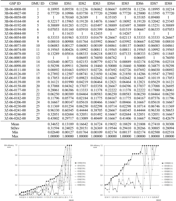
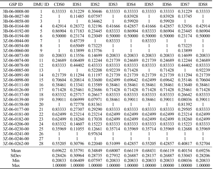
For 28 DMUs in <Table 3>, DEA efficiency scores are summarized in <Table 5> by the CCR-I (input-oriented CCR) model Eq. (2) and <Table 6> shows another DEA effi- ciency scores by the BCC-I (input-oriented BCC) model Eq.
(3). Meantime, Park et al. (2011), summarized some public R&D performance efficiency evaluation studies using vari- ous input-oriented DEA models. In addition, Paradi et al.
(2004), presented a table of DEA orientation possibilities as- sociated with the three approach perspectives (i.e., produc- tion, profitability and intermediation) which shows that in- put-oriented DEA models can be used for the three approach perspectives. Based on the literature mentioned above, the present study adopts an input-oriented DEA model. <Table 5> shows nine different series of DEA efficiency scores; the first one is obtained using CDS0. The rest of the eight series correspond with IDS1 to IDS8 respectively. In the column of CDS0, three DMUs-DMU ID 3, 7, 13-are efficient. Howe- ver, in the column of CDS0 in <Table 6>, the number of effi- cient DMUs is nine (DMU ID 2, 3, 7, 8, 9, 13, 20, 26, 27), which can be regarded as an effect of VRS assumption (DEA-Solver-Pro 2012 ).
<Figure 4> visualizes DEA efficiency scores in <Table 5>, sorted by CDS0 ascending order for the comparisons of nine different data structures in <Figure 3> Also, <Figure 5> is presented to depict <Table 6> in a similar manner. In both
<Figure 4> and <Figure 5>, it can be seen that the series of CDS0 is greater than or equal to the remaining eight IDSs.
That can be interpreted as a natural behavior of DEA caused by “the space dimensionality” mentioned by Seiford and Thrall (1990).
4.2 Finding Highly Correlated Data Structures
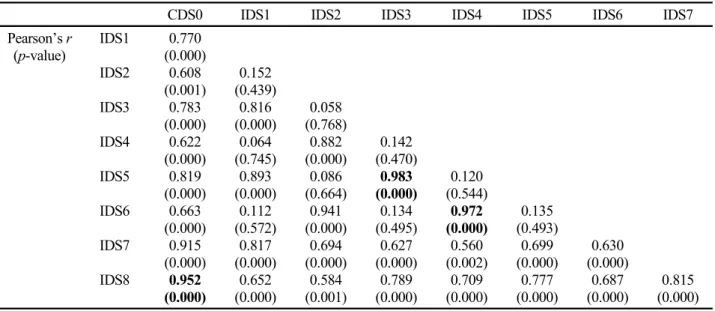
Here, some interesting facts are found. Actually, there are
some highly positive (+) correlations detected between CDS0
and a few IDSs. First, in <Table 7>, r = 0.394 (p-value =
0.038) is the lowest between CCR-I and BCC-I efficiency
scores associated with (1×1) IDS3 ( → ). This means
Table 5. DEA efficiency scores of CCR-I model
GSP ID DMU ID CDS0 IDS1 IDS2 IDS3 IDS4 IDS5 IDS6 IDS7 IDS8
3B-06-0008-00 3B-06-0027-00 3B-06-0058-00 3B-06-0164-00 3B-06-0192-00 3B-06-0194-00 3Z-06-0044-00 3Z-06-0054-00 3Z-06-0060-00 3Z-06-0073-00 3Z-06-0074-00 3Z-06-0078-00 3Z-06-0085-00 3Z-06-0091-00 3Z-06-0098-00 3Z-06-0111-00 3Z-06-0126-00 3Z-06-0137-00 3Z-06-0139-00 3Z-06-0158-00 3Z-06-0177-00 3Z-06-0181-00 3Z-06-0182-00 3Z-06-0206-00 3Z-06-0230-00 3Z-06-0241-00 3Z-06-0246-00 3Z-06-0262-00
1 2 3 4 5 6 7 8 9 10 11 12 13 14 15 16 17 18 19 20 21 22 23 24 25 26 27 28
0.18995 0.77720
1 0.32217 0.38889 0.07053
1 0.33333 0.08810 0.06083 0.19565 0.13289
1 0.02640 0.58298 0.08892 0.27892 0.17053 0.16121 0.37088 0.28061 0.06250 0.11796 0.16667 0.11369 0.96330 0.32051 0.43802
0.09558 0.10906 0.70160 0.15965 0.01283 0.01160 0.11633 0.01963 0.00988 0.00127 0.00426 0.05816
1 0.00721 0.09911 0.01663 0.12507 0.01457 0.01990 0.04362 0.06386 0.00389 0.05774 0.00147 0.01254 0.60345 0.02684 0.29717
0.11236 0.03750 0.26389 0.19120 0.15251 0.05910
1 0.33333 0.01764 0.06083 0.10992 0.08333 0.06693 0.02153 0.28694 0.05015 0.08741 0.09823 0.04219 0.37037 0.13333 0.04464 0.02184 0.05618 0.06250 0.44444 0.32051 0.13089
0.06062 0.77720
1 0.14876 0.03497 0.01399 0.12435 0.01679 0.03992 0.00109 0.00811 0.06218 0.76050 0.00779 0.18460 0.02726 0.21850 0.02642 0.06464 0.03358 0.11378 0.00583 0.11775 0.00466 0.02298 0.38705 0.01492 0.40449
0.06667 0.25000 0.35185 0.16667 0.38889 0.06667
1 0.26667 0.06667 0.04861 0.19565 0.08333 0.04762 0.02174 0.50000 0.07692 0.14286 0.16667 0.12821 0.26667 0.22222 0.06250 0.04167 0.16667 0.10714 0.26667 0.16667 0.16667
0.09558 0.77720
1 0.18092 0.03497 0.01519 0.14267 0.02113 0.03992 0.00137 0.00811 0.07133
1 0.00889 0.18460 0.02726 0.21850 0.02642 0.06464 0.04396 0.11378 0.00583 0.11775 0.00466 0.02298 0.60345 0.02684 0.41406
0.11236 0.25000 0.35185 0.19120 0.38889 0.06667
1 0.33333 0.06667 0.06083 0.19565 0.08333 0.06693 0.02174 0.50000 0.07692 0.14286 0.16667 0.12821 0.37037 0.22222 0.06250 0.04167 0.16667 0.10714 0.44444 0.32051 0.16667
0.18995 0.13595 0.89480 0.32042 0.15251 0.06355
1 0.33333 0.02500 0.06083 0.10992 0.12891
1 0.02596 0.34875 0.06030 0.19547 0.10119 0.05629 0.37088 0.17880 0.04464 0.07376 0.05618 0.06746 0.96330 0.32051 0.39602
0.10214 0.77720
1 0.25345 0.38889 0.07053
1 0.26667 0.08810 0.04861 0.19565 0.11845 0.76050 0.02518 0.58298 0.08892 0.27892 0.17053 0.16121 0.26695 0.28061 0.06250 0.11796 0.16667 0.11369 0.50653 0.16667 0.42679 StDev Mean
Min Max
0.34652 0.31594 0.02640 1.00000
0.13189 0.24025 0.00127 1.00000
0.16642 0.20151 0.01764 1.00000
0.16724 0.26369 0.00109 1.00000
0.19652 0.19544 0.02174 1.00000
0.18829 0.29410 0.00137 1.00000
0.21808 0.20266 0.02174 1.00000
0.27410 0.30885 0.02500 1.00000
0.30308 0.28094 0.02518 1.00000
DEA efficiency score
DMUID Sorted by CDS0(CCR-1) ascending order
Figure 4. DEA efficiency scores sorted by CDS0 (CCR-I) ascending order
DEA efficiency score
DMUID Sorted by CDS0(CCR-1) ascending order
Figure 5. DEA efficiency scores sorted by CDS0 (BCC-I) ascending order
that those two variables and y1 are more sensitive to VRS constraint in Eq. (4) than the other two variables and . In other words, and are inactive in calculating BCC-I efficiency score.
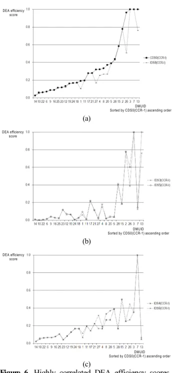
For a more detailed analysis of the determinants identi- fication, <Figure 4> is separated into three distinct panels in
<Figure 6> and each panel is comprised of the series having
highly positive (+) correlations in <Figure 4>. Similarly,
Table 6. DEA efficiency scores of BCC-I model
GSP ID DMU ID CDS0 IDS1 IDS2 IDS3 IDS4 IDS5 IDS6 IDS7 IDS8
3B-06-0008-00 3B-06-0027-00 3B-06-0058-00 3B-06-0164-00 3B-06-0192-00 3B-06-0194-00 3Z-06-0044-00 3Z-06-0054-00 3Z-06-0060-00 3Z-06-0073-00 3Z-06-0074-00 3Z-06-0078-00 3Z-06-0085-00 3Z-06-0091-00 3Z-06-0098-00 3Z-06-0111-00 3Z-06-0126-00 3Z-06-0137-00 3Z-06-0139-00 3Z-06-0158-00 3Z-06-0177-00 3Z-06-0181-00 3Z-06-0182-00 3Z-06-0206-00 3Z-06-0230-00 3Z-06-0241-00 3Z-06-0246-00 3Z-06-0262-00
1 2 3 4 5 6 7 8 9 10 11 12 13 14 15 16 17 18 19 20 21 22 23 24 25 26 27 28
0.33333 1 0.42914 1 0.86904 0.50000
1 1 1 0.20833 0.24689 0.83333 0.21739 1 0.70604 0.38461 0.71428 0.83332 0.39011
1 0.83333 0.62499 0.62499 0.83332 0.35969
1 1 0.55205
0.31229 0.11485 0.28372 1 0.17183 0.23174 0.45739 0.65049 0.13899 0.13556 0.06409 0.44402 0.11294 1 0.20814 0.13341 0.25461 0.25717 0.06999 0.72778 0.27307 0.23214 0.18260 0.14607 0.11055
1 1 0.30796
0.30446 0.07597 0.34462 0.32196 0.23445 0.23049
1 0.73225 0.13756 0.14699 0.12244 0.43333 0.52208 0.11197 0.33600 0.13589 0.23686 0.26617 0.07971 0.81361 0.29290 0.23214 0.17038 0.15223 0.12661 0.97634 0.22040 1
0.33333 1 0.41666 1 0.83333 0.50000 0.83333
1 1 0.20833 0.21739 0.83333 0.92239 0.21739 0.62499 0.38461 0.71428 0.83333 0.38461
1 0.83333 0.62499 0.62499 0.83333 0.35714
1 1 0.51099
0.33333 0.83928 0.59920 0.42857 0.86904 0.50000
1 1 1 0.20833 0.24689 0.83333 0.71428 0.21739 0.69642 0.38461 0.71428 0.83333 0.39011
1 0.83333 0.62499 0.62499 0.83333 0.35969
1 1 0.42857
0.33333 1 0.41666 1 0.83333 0.50000 0.83333
1 1 0.20833 0.21739 0.83333 0.21739 1 0.62499 0.38461 0.71428 0.83333 0.38461
1 0.83333 0.62499 0.62499 0.83333 0.35714
1 1 0.55205
0.33333 0.83928 0.59920 0.42857 0.86904 0.50000
1 1 1 0.20833 0.24689 0.83333 0.71428 0.21739 0.69642 0.38461 0.71428 0.83333 0.39011
1 0.83333 0.62499 0.62499 0.83333 0.35969
1 1 0.42857
0.31229 0.13745 0.32936 1 0.23445 0.23174
1 0.73225 0.13899 0.14699 0.12244 0.44402 0.11294 1 0.35146 0.13640 0.25461 0.26642 0.08036 0.81392 0.29505 0.23214 0.18260 0.15223 0.12688
1 1 0.40817
0.33333 1 0.42914 1 0.86904 0.50000
1 1 1 0.20833 0.24689 0.83333 0.92239 0.21739 0.70604 0.38461 0.71428 0.83333 0.39011
1 0.83333 0.62499 0.62499 0.83333 0.35969
1 1 0.52704 StDev Mean
Max Min
0.69622 0.28426 0.20833 1.00000
0.35791 0.30964 0.06409 1.00000
0.34849 0.28735 0.07597 1.00000
0.68007 0.27932 0.20833 1.00000
0.66119 0.26887 0.20833 1.00000
0.68431 0.28137 0.20833 1.00000
0.66119 0.26887 0.20833 1.00000
0.40154 0.33043 0.08036 1.00000
0.69256 0.28206 0.20833 1.00000 Table 7. Correlation coefficients of DEA efficiency scores between CCR-I and BBC-I model
CDS0 IDS1 IDS2 IDS3 IDS4 IDS5 IDS6 IDS7 IDS8 Min Max
Pearson’s r
(p-value) 0.606
(0.001) 0.702
(0.000) 0.809
(0.000) 0.394
(0.038) 0.434
(0.021) 0.435
(0.021) 0.517
(0.005) 0.882
(0.000) 0.550
(0.002) 0.394 0.882
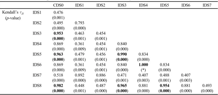
<Figure 7> has two panels that are extracted from <Figure 5> In the preparation of <Figure 6> and <Figure 7>, each panel has the series that satisfy their correlation coefficient
≥ 0.950 (p-value ≤ = 0.05) in <Table 8> and <Table 9>.
In particular, determinants are more clearly identified in
<Figure 7> and <Table 9>, associated with the BCC-I model.
From <Figure 7>(a), it can be seen that four distinct data structures-CDS0, IDS3, IDS5 and IDS8-generate approximately identical DEA efficiency scores. Furthermore, <Figure 7>(b) reveals that IDS4 and IDS6 generate exactly the same DEA efficiency scores. Two common variables are “R&D manpower”
( ) and “Sales revenue” ( ), shared by the four data struc- tures in <Figure 7>(a). Conversely, the other two variables,
“R&D funds” ( ) and “New employment” ( ), are in-
active or insignificant in calculating DEA efficiency scores whether or not they are included in the four data structures.
Also, the sole difference between (1×1) IDS4 ( → ) and (2 × 1) IDS6 ( and → ) is the presence or absence of
“R&D funds” ( ). It implies again that “R&D funds” ( ) is a thoroughly insignificant variable.
As for the CCR-I model, <Figure 6> presents three panels.
<Figure 6>(a) has two series of DEA efficiency scores-CDS0 and IDS8 and <Figure 6>(b) has another two series-IDS3 and IDS5. Therefore, it is seen that <Figure 7>(a) is just split into two panels as per <Figure 6>(a) and <Figure 6>(b). In sum- mary, <Figure 6> and <Figure 7> accompanied by <Table 8>
and <Table 9> prove clearly that the two determinants are
“R&D manpower” ( ) and “Sales revenue” ( ) and the
DMUID
Sorted by CDS0(CCR-1) ascending order DEA efficiency
score
(a)
DEA efficiency score
DMUID
Sorted by CDS0(CCR-1) ascending order
(b)
DEA efficiency score
DMUID
Sorted by CDS0(CCR-1) ascending order
Figure 6. Highly correlated DEA efficiency scores (c) sorted by CDS0 (CCR-I) ascending order
DMUID Sorted by CDS0(BCC-1) ascending order DEA efficiency
score
(a)
DMUID Sorted by CDS0(BCC-1) ascending order DEA efficiency
score