평균 형상 모델과 SIFT 특징을 이용한 TRUS 영상의 전립선 분할 187
KIPS Tran Softw Data Eng
A Prostate Segmentation of TRUS Image using Average Shape Model and SIFT Features
Sang Bok Kim
†․Yeong Geon Seo
††ABSTRACT
Prostate cancer is one of the most frequent cancers in men and is a major cause of mortality in the most of countries. In many diagnostic and treatment procedures for prostate disease, transrectal ultrasound(TRUS) images are being used because the cost is low. But, accurate detection of prostate boundaries is a challenging and difficult task due to weak prostate boundaries, speckle noises and the short range of gray levels. This paper proposes a method for automatic prostate segmentation in TRUS images using its average shape model and invariant features. This approach consists of 4 steps. First, it detects the probe position and the two straight lines connected to the probe using edge distribution. Next, it acquires 3 prostate patches which are in the middle of average model. The patches will be used to compare the features of prostate and nonprostate. Next, it compares and classifies which blocks are similar to 3 representative patches.
Last, the boundaries from prior classification and the rough boundaries from first step are used to determine the segmentation. A number of experiments are conducted to validate this method and results showed that this new approach extracted the prostate boundary with less than 7.78% relative to boundary provided manually by experts.
Keywords : Prostate, Average Model, Prostate Segmentation, TRUS Prostate
평균 형상 모델과 SIFT 특징을 이용한 TRUS 영상의 전립선 분할
김 상 복
†․서 영 건
††요 약
전립선암은 남자에게 가장 흔히 나타나는 암 중의 하나이며, 많은 나라에서 죽음에 이르게 하는 큰 요인이 되고 있다. 전립선암을 진단하고 치료하는 과정에서 비용이 싼 TRUS 영상이 사용된다. 그러나 전립선 경계의 정확한 구분이 요구되지만 어려운 문제이다. 그 이유는 경계가 불 명확하고, 반점들이 많으며, 그레이 레벨의 범위가 작기 때문이다. 본 연구에서는 전립선의 평균 형상 모델과 불변의 특징을 이용하여 TRUS 영상에서 자동으로 전립선 분할하는 방법을 제안한다. 이 방법은 4 단계로 구성된다. 먼저, 에지 분포를 이용하여 프로브와 두개의 직선을 찾아 낸다. 다음으로, 평균 형상 모델의 중앙에 위치한 3개의 전립선 패치를 획득한다. 이 패치는 전립선과 비전립선의 특징을 비교하기 위해 사용된 다, 다음으로, 세 개의 패치와 각 블록들이 얼마나 대표 블록과 유사한지를 비교한다. 마지막으로, 앞 단계의 경계와 첫 단계에서 얻은 개략적 경계가 최종 분할에 사용된다. 이 방법의 유효성을 검증하기 위하여 실험을 하였으며, 인간 전문가에 의해 얻어진 경계와 비교하여 7.78% 미만 의 차이로 경계를 얻을 수 있었다.
키워드 : 전립선, 평균 모델, 전립선 분할, 초음파 전립선
1. Introduction 5)
In the united states, prostate cancer is the most frequently diagnosed cancer in men and the second cancer-related cause of death for them [1,2]. According to the American Cancer Society, dead rate is decreasing
†정 회 원 : 경상대학교 컴퓨터과학과 교수, 컴정통신연구소원
††종신회원 : 경상대학교 컴퓨터과학과 교수, 컴정통신연구소원 논문접수 : 2012년 9월 3일
수 정 일 : 1차 2012년 10월 15일 심사완료 : 2012년 10월 18일
* Corresponding Author : Yeong Geon Seo([email protected])
every year caused by prostate cancer, but it is 23 per 100,000 people in 2007[3]. The rate is second highest value following the dead rate of lung and bronchus.
Ultrasound imaging is a widely used technology for diagnosing and treatment this kind of cancer [4].
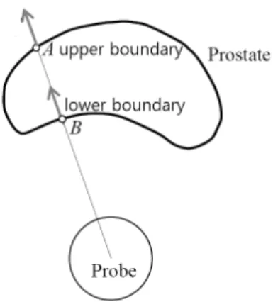
Especially, transrectal ultrasound (TRUS) prostate images are captured more easily and with lower cost. In fig. 1, an example of TRUS image capture is shown[1].
US(Ultrasound) imaging is the main modality for prostate cancer diagnosis and treatment, due to many of its clinical advantages, expensive and easy to use.
http://dx.doi.org/10.3745/KTSDE.2012.1.3.187
Fig. 1. Placements of human organs and US probe
Fig. 2. (a) center image (b) base image (c) apex image Accurate segmentation of prostate boundaries from US
images plays an important role in many prostate-related applications such as the accurate placement of the needles and biopsy, the assignment of the appropriate therapy in cancer treatment, and the measurement of the prostate gland volume [5]. Moreover, the shape of the prostate in US images is considered as an important indicator for staging prostate cancer. But, because the boundaries between prostate and nonprostate of the image are ambiguous, an automatic extraction of the boundaries has some difficulties [6,7]. Such that, they are very weak texture structure, low contrast, fuzzy boundaries, speckle noise and shadow regions. To cope with these problems, different methods have been studied.[6] developed a deformable segmentation using Gabor-support vector machine based 3D prostate images. [8] presented a new paradigm for the edge-guided delineation, providing the algorithm-detected prostate edges as a visual guidance for the user to manually edit. [9] designed a statistical shape model for outlining prostate boundary from 2D TRUS images. [10] presented a level set based method to detect prostate surface from 3D US images. [11] proposed an automatic segmentation for the prostate from 2D TRUS using adaptive learning local shape statistics. [12]
presented an automatic segmentation of the prostate in 3D TRUS images by extracting texture features and by statistically matching geometrical shape of the prostate.
To classify more precisely the boundaries between prostate and nonprostate, this study proposes an approach using average prostate model and modified SIFT(Scalar Invariant Feature Transform)[13], and consists of 4 steps.
In first step, it detects the probe position, the two straight lines connected to the probe, and rough boundaries between prostate and nonprostate using edge distribution. Here, the boundaries are never fully
connected as the edges are difficult to be clearly classified, so they will be used in last step. In second step, it acquires 3 prostate patches which are in the middle of average model. The patches will be used to compare the features of prostate and nonprostate. In third step, after extracting the features from the 3 patches, and the features from the whole images divided by block, it compares and classifies which blocks are similar to 3 representative patches. In last step, the boundaries from prior classification and the rough boundaries from first step are used to determine the segmentation. The results experimented from our method made difference by 9.7%
compared to one of human expert.
2. Related Studies
In this chapter, we present difficulties of US prostate segmentation, existing approaches and then SIFT.
2.1 US prostate
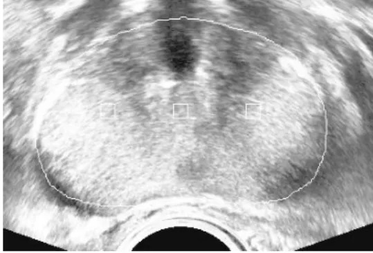
US prostate image has a lot of noise and is hard to delineate the boundaries as you can see in fig. 2 Especially, the base and apex parts of prostate are generally unclear or broken, since these boundaries are almost parallel to US beams of the transducer. Therefore, the images of the two parts are almost impossible to delineate the boundaries without reference of their neighbor’s boundaries.
Several methods were proposed for the above
problems. First, [4,6] proposed a deformable segmentation
method. The boundaries of deformable model is
subsequently driven to the boundary between the
tentatively labeled prostate and nonprostate tissues, while
its shape is limited by pre-constrained shape. Tentative
tissue labeling and subsequent deformation are repeated
until they converge to the boundary in the prostate
images. [11] proposed an automatic segmentation for the
prostate from 2D TRUS using adaptive learning local
shape statistics. Another method is to use 3D
segmentation [6,12]. Using 3D image the method gets the
KIPS Tran Softw Data Eng Fig. 4. (a) Different delineated prostate shapes and
(b) Average prostate shape model statistical boundary model from apex to base. The
boundaries of an image are adjusted within a certain limit of the pre-acquired 3D model. Disadvantages of these methods can’t find abnormal protrusions like tumor.
Fig. 3. Relation between the position of probe and the shape of prostate
2.2 Distribution depending on probe
US probe scans the objects with fan shape like fig. 2.
So, the shape of prostate has no choice to be chestnuts.
Also, the US probe that was used to capture TRUS images appears as dark disc. Therefore, the location and the radius of the US probe can be easily detected.
Prostate is two parts of boundaries, i.e. upper boundary and lower boundary. The lower boundary is always close to the probe, which results from the acquisition procedure of images. The rough position of the prostate relative to the probe can be represented by the orientation of a line connecting the centers of the probe and the prostate, which can be used for initialization of the prostate model.
Generally most prostate segmentation approaches first detect the location of the probe and then use the location of the probe to roughly estimate the location of the prostate since they have a strong relationship. At same time, the two straight lines which are connected to both ways of the probe can be detected to estimate more precisely the position and shape of the prostate. Original shape of prostate is like eggs or potatoes, which can be acquired by CT or MRI, but the shape from US is one of beans like fig. 3.
2.3 Average prostate shape model
Average shape model is important to roughly estimate the shape of the prostate[9]. Fig. 4 shows an example of the average shape acquired from expert's boundaries. The human experts are required to outline image to give an initialization model. The diversity and complexity of
anatomical shapes guides the shape model and allowable variation. There are several shape models, point distribution, active shape, active appearance model, Fourier snakes, active contours, and Parametrically deformable model. Point distribution model represents a shape instance by a judiciously chosen set of point (features), each of which is k-dimension vector. In the simplest case p
i=(x
i, y
i) and k=2, {p
i: i = 1,..,n}. The n feature point are stacked into a long vector of length kn.
To find a model instance in an image, it needs to comprise the average shape and set of t modes. This presents with a new image and tries to fit the shape model to the image. And this requires both that we find the appropriate weight that define the model instance and that we find the transformation from shape space to the image, to align the model instance with the image.
2.4 SIFT
SIFT[13] has an algorithm to extract the features invariant the scale and orientation of image. The advantages are powerful to image scale, illumination, movement, rotation and occlusion. It has 4 steps, scale-space extrema detection, keypoint localization, orientation assignment, and keypoint descriptor. First step determines the scale and position of the features. Such that, it extracts some interest points which their scale and orientation are supposed to be invariant. To do this, it needs Gaussian pyramid, which uses DoG(Difference of Gaussian).
⊗ (1)
(2)
Where, G(x, y) is Gaussian filter.
Fig. 5. From image gradient to keypoint descriptor
img = LoadImg(filename) ;
shape_model = LoadAveShapeModel() ; [probe, straight_line] = GetProbeLines(img) ; model_pos = ApplyShapelModel(shape_model,
probe, straight_line) ; descriptor = ModifiedSIFT(img) ;
dist_table = CompareImg(descriptor, model_pos);
final_bound = AdjustBoundary() ;
function ModifiedSIFT(img)
gauss = GaussianTransform(img) ; while existing block
center_pt = GetCenterfromEachBlock() ; [scale, space] = Diff(gauss, center_pt) ; descriptor[] = ComputeDescriptor(scale,
space) ; end
end
function LoadAveShapeModel() return(shape_model_img_file) ; end
Fig. 6. Overall procedures
Fig. 7. A sample image and its background Second step erases the points which are not good for
extracting features. Such that, of the points used as the candidates of the keypoint, non stable points are erased for matching, and the keypoints are precisely positioned in continuous space. For this, SIFT uses Taylor series.
Third step determines directions, magnitudes and orientations of the keypoints' neighbors using next two equations, and then makes orientation histogram.
(3)
tan
(4)
In last step, it presents the features again, such that, gets orientation of the gradient values neighboring the keypoints. After processing SIFT, keypoint descriptors from image gradients are generated like fig. 5.
3. Delineating the boundary of prostate
To classify the prostate region from its background, we use average prostate model and scale and orientation invariant feature transform using modified SIFT, and then adjustment using the model and invariant features.
3.1 Overall procedures
Like fig. 6, the approach consists of preprocessing, getting probe and two straight lines which will be used to pose the average prostate model and to get sample prostate blocks, applying average prostate model that uses the predefined average model mentioned in 2.3, scale invariant feature transform which makes descriptors using predefined keypoints, getting prostate sample blocks which are acquired in the center of the model, comparing sample block and others which roughly discriminates
prostate blocks and nonprostate blocks, and finally adjusting the boundary using the model and roughly discriminated blocks.
3.2 Getting probe and two straight lines
Preprocessing step consists of histogram equalization, so that the histogram of the output approximately matches a specified histogram, stick filtering which filters to reduce the speckle noise, morphological filtering which is used to smooth filtered image and enhanced contrast near edges, and finally getting background which will be used to be excluded for training. Fig. 7 shows a sample prostate image and its useless region which is black.
Next, to get two straight lines like fig. 8, it needs to
mask the image using 10-direct masks which are
KIPS Tran Softw Data Eng Fig. 9. Average model and Image put the model
Fig. 10. Position of 3 sample prostate blocks in the center of the model
Fig. 11. Prostate distribution after comparing sample prostate blocks and other blocks
. Using the masks, it can 10-direct edges and get two straight lines. And then the probe always is between the two lines. To get more accurate probe(arc) equation and its position, it needs to compute two cross points between the arc and two lines.
The cross points, probe's potion, two straight lines are shown in fig. 8.
Fig. 8. Probe and two straight lines after edge detection
3.3 Applying average prostate shape model
The existing average prostate shape is similar to the figure of fig. 4, but we use the model of fig. 9. Our defined model is closer to average shape of prostate. To pose the shape on the test image, we adjust its center position like equation (5) and (6), and to resize the shape, we adjust it like equation (7). x coordinate of the center of the model is same as x coordinate of the probe in the image and y coordinate of the center of the model is above 2.8 times from the center of the probe. The size of the model is 4.5 times of the radius of the probe. After resizing and posing the shape, you can see the image in fig. 9.
center_of_x = center_of_probe_x (5) center_of_y = center_of_probe_y - probe_radius * 2.8 (6) size_of_model = probe_radius * 4.5 (7)
3.4 Modified SIFT
To find the features invariant to scale and orientation, we use modified SIFT. To compare which blocks belong to prostate region or nonprostate region, whole image is divided with 16x16 blocks. Each divided block will be compared to 3 sample prostate blocks which come from 3 centers of the average shape position like fig. 10. As described in 2.4, each block are transformed by Gaussian scale and space, and then difference of scale and space are generated from it. After doing them, each block's orientation and descriptor are obtained. Generally this process in other studies needs keypoints, but our approach only uses one center point of the block to compare among same sized blocks.
3.5 Comparing sample blocks and others
This step compares 3 prostate sample blocks and other blocks divided with 16x16 how much similar two different groups are. 3 sample blocks are considered as prostate block. All transformed blocks have their keypoint descriptors which consists of 128 real numbers for the center point of each block. The blocks are 16x16 size, but duplicated as 50%. That is, its step size is not 16, but 8.
If the image size is 128x128, the number of blocks is 256
(b) image2
(c) image3
Fig. 13. Positions of probe and two straight lines(left) and average shape model of each image(middle), and final
segmentation results(right) (a) image1 to compare more accurately. Like fig. 10, after obtaining 3
prostate sample blocks which are in the center of the model, all other blocks are compared with sample blocks 3 times. The result values mean whether a block is similar or not to the prostate sample blocks. If a block is similar to 2 of 3 sample blocks, the block is regarded as prostate, otherwise nonprostate. As you can see in fig. 11, the prostate can be in the region of nonprostate, and the nonprostate can be in one of prostate. White blocks mean prostate and black ones mean nonprostate.
3.6 Adjusting the boundary
Before adjusting the boundary, noises have to be erased.
The noises means the groups apart from the center prostate blocks. And then, adjusting the boundary is done by projecting all the contour blocks onto the local regression line. Here, each contour block has contour points which meet with nonprostate blocks. For each point, N neighboring points which lie on the contour are sampled on each side and a local regression line is computed. Then the current point is projected on this line. Applying this algorithm to all the points smooths the contour and in a way brings the points closer. 2N+1 is the number of total points contributing to the computation of the local regression line. The higher the number of points are , the smoother the curve is. Because of the linear nature of fitting, when too much smoothing is desired, some important features such as protrusions may be loosed. This way is a wrong over-smoothing. A way to be less prone to such errors is to use Gaussian weighted least squares fit. Fig. 12 shows the prostate after erasing noises and adjusting the boundary from fig. 11.
Fig. 12. Prostate boundary after adjusting the boundary
4. Experimental Results and Analysis
This study uses experimental results comparing the difference of boundaries between human expert and our
method. Additionally, we show the results of the processes mentioned in chapter 3.
4.1 Processes of segmentation
We show whether the proposed method is applied to different prostate images properly or not. First. getting probe and two straight lines, applying average shape model, and after applying scale and orientation invariant transform, finally we show the result from adjusting the boundary. To show experimental result, we shows only three images of several images.
In fig. 13, the left images present the positions of probe(round shape of the center) and two straight lines, the middle images present the positions of average shape(white solid line) put over the image and the right images present final segmentation result after adjusting.
The average shape is depended on the probe and two lines of the image. As seeing in the figure, we can see what the shapes are well positioned and the prostate boundaries are well segmented.
4.2 Comparisons of objective and subjective views
Actually, even human experts have difference of their
drawn boundaries because they can not precisely delineate
KIPS Tran Softw Data Eng methods
test images
proposed method
[6]
method
[11]
method
[12]
method
image1 7.63 7.90 8.02 7.63
image2 7.78 7.70 7.93 7.75
image3 6.57 7.02 7.54 6.70
Table 1. Differential values between human expert and the proposed method and the existing methods (%) the boundaries between the prostate and nonprostate.
Especially, because the apex image and base image have a lot of noises, the precise boundary has some variation with ±5%. In the right images of fig. 14, the solid line is the boundary by the proposed method. For subjective comparison, we used difference between two boundaries of the proposed method and human expert. Such that, the difference(D) comes from the following equation(8).
D = count(for all pixels E(x, y) and P(x,y), labels(E(x,y)!=P(x,y))) / count(prostate of E) (8)
Here, E means expert and P means the proposed method. Table 1 shows the results of differential values between human expert and diverse methods on delineating the boundary. Fig. 14 shows the results classified by each method, it is hard for people to identify which one is better than others. These results of [6], [11]
and [12] are gotten from executing the executable program which have their method. The reason why our method is superior than the existing methods is that we applied SIFT to classify more clearly the features of prostate and nonprostate.
Fig. 14. Overall experimental results, expert boundary(dotted line), the proposed method(solid line), [6] method(+), [11]
method(x) and [12] method(o)
5. Conclusion
This paper proposed a TRUS prostate segmentation using average shape model and invariant features Average shape model is acquired from average prostate positions and shapes of 20 prostate images. Invariant feature used an algorithm to extract the features invariant the scale and orientation of image. Our method was similar or better(0.45%) than the existing method in terms of the difference of prostate boundary between human expert and our method. Our future studies are to improve the computation time, to apply human expert's knowledge, and finally to implement 3D segmentation and modeling.
References
[1] Cancer Facts and Figures. American Cancer Society.
http://www.cancer.org.
[2] Mettlin C: American society national cancer detection project.
Cancer 1995, 75:1790-1794.
[3] http://www.cancer.org/Research/CancerFactsFigures/Cancer act/cancer-facts-figures-2011.
[4] A. Chakraborty, L. H. Staib, and J. S. Duncan, “Deformable Boundary Finding in Medical Images by Integrating Gradient and Region Information”, IEEE Trans. Med. Imag., Vol.15, No.6, pp.859–870, Dec.,1996.
[5] P. D. Grimm, J. C. Balsko, and H. Ragde, “Ultrasound Guided Transperineal Implantation of Iodine 125 and Palladium 103 for the Treatment to Fearly Stage Prostate Cancer”, Atlas Urol. Clin. No. Amer., Vol.2, pp.113–125, 1994.
[6] Y. Zhan and D. Shen, “Deformable Segmentation of 3-D Ultrasound Prostate Images Using Statistical Texture Matching Method”, IEEE Trans. on Medical Imaging, Vol.25, pp.245-255, March, 2006.
[7] A. Rafiee, A. Salimi, and A. Roostam, “A Novel Prostate Segmentation Algorithm in TRUS Images”, World Academy of Science, Engineering and Technology 45, pp.120-124, 2008.
[8] S. D. Pathak, V. Chalana, D. R. Haynor, and Y. Kim,
“Edge-guided Boundary Delineation in Prostate Ultrasound Images”, IEEE Trans. Med. Imag., Vol.19, No.12, pp.1211–
1219, Dec., 2000.
[9] D. Shen, Y. Zhan, and C. Davatzikos, “Segmentation Prostate Boundaries from Ultrasound Images Using Statistical Shape Model”, IEEE Trans. Med. Imag., Vol.22, No.4, pp.539–551, Apr., 2003.
[10] F. Shao, K. V. Ling, and W. S. Ng, “3-D Prostate Surface
Detection from Ultrasound Images Based on Level Set
Method”, Proc. MICCAI 2003, pp.389–396, 2003.
[11] P. Yan, S. Xu, B. Turkbey and J. Kruecker, “Adaptively Learning Local Shape Statistics for Prostate Segmentationin Ultrasound”, IEEE Trans. On Biomedical Engineering, Vol.58, No.3, pp.633-641, Mar., 2011.
[12] H. Akbari, X. Yang, L. Halig and B. Fei, “3D Segmentation of Prostate Ultrasound Images Using Wavelet Transform”, Proc. of SPIE 7962, 2011.
[13] B. E. Boser, I. M. Guyon and V. N. Vapnik. “A Training Algorithm for Optimal Margin Classifiers”, In D. Haussler, editor, 5th Annual ACM Workshop on COLT, pp.144–152, 1992.
[14] J. Suri and A. Farag, “Deformable Models 2”, Springer, pp.75-94, 2007.
[15] A. Ghanei, H. Soltanian-Zadeh, A. Ratkesicz, and F. Yin,
“A Three-Dimensional Deformable Model for Segmentation of Human Prostate from Ultrasound Image”, Med. Phys., Vol.28, pp.2147–2153, 2001.
김 상 복
e-mail : [email protected]
1989년 중앙대학교 전자공학과(박사) 1984년~현 재 경상대학교 컴퓨터과학과 교수
2001년~현 재 경상대학교 컴퓨터정보 통신연구소원
관심분야 : 멀티미디어통신, 영상인식, 보안
서 영 건


![Fig. 14. Overall experimental results, expert boundary(dotted line), the proposed method(solid line), [6] method(+), [11]](https://thumb-ap.123doks.com/thumbv2/123dokinfo/5258020.630779/7.892.120.398.707.1088/overall-experimental-results-expert-boundary-dotted-proposed-method.webp)
