IEG 환경지질연구정보센터

전체 글

(1). Geosciences Journal Vol. 8, No. 1, p. 27 42, March 2004. Application of representative elementary area (REA) to lineament density analysis for groundwater implications Gyoo-Bum Kim Jin-Yong Lee Kang-Kun Lee*. Groundwater Investigation Sec., Korea Water Resources Corporation, Daejon 306-711, Korea GeoGreen21 Co., Ltd., Suite 519, Innovation Center, Research Park, Seoul National University, Seoul 151-818, Korea School of Earth and Environmental Sciences, Seoul National University, Seoul 151-742, Korea. ABSTRACT: Lineament density maps can be used for the quantitative evaluation of relationships between lineaments and the occurrence of groundwater. This paper reports the usefulness of the representative elementary area (REA) concept for lineament analysis. This concept refers to the area of the unit circle needed to calculate the lineament density factors distributed within the circle: length, counts and cross-points counts. The circle is a unit circle where one calculates the sum of the lineament length, lineament counts and the number of cross-points within it. The REA is needed to obtain the best representative lineament density map prior to the analysis of relation between lineaments and groundwater well yield or other groundwater characteristics. A lineament map for the Yongsangang-Seomjingang watershed of Korea was used for demonstrating the concept. It is shown that the REA concept can be efficiently applied to lineament density analysis and mapping. In the demonstration case, the lineament densities are inversely proportional to the size of the REA, and the REA can be calculated with this inversely linear regression model. If the average lineament density values for the whole study area are known, the most accurate density maps can be drawn using the REAs obtained from each linear regression model. Key words: lineaments, lineament length density, lineament crosspoints density, lineament counts density, linear regression model. 1. INTRODUCTION Lineaments obtained from remote sensing data or airborne photographs have usually been used in groundwater exploration or investigations. Currently, groundwater development in Korea is mostly from fractures or joints in the deep bedrock aquifer, so the analysis and interpretation of lineaments are very important. Because lineaments may play an important role in groundwater flow and contaminant transport in the deep aquifer, they provide important information for planning management strategies, including determination of areas where groundwater resources need protection. Lineament extraction and analysis have been studied by Caponera (1989), Koike (1995), Mah et al. (1995), Karnieli et al. (1996), Kim et al. (1999), Park et al. (2000), Casas et al. (2000) and Costa et al. (2001). They all emphasized that lineaments are closely related to groundwater occurrence because the lineaments are formed mechanically by frac*Corresponding author: [email protected]. tures, faults, joints, dykes, rock boundaries and folds that can provide groundwater flow paths. In particular, Casas et al. (2000) defined the best fitting cell size by calculating the distance between neighboring lineaments based on the Delauney triangulation method. They produced a lineament-length density map by applying the best-fit size to their study area and found that if the grid became larger or smaller than the optimum size, the density maps did not efficiently reflect the geological features. The density of lineament lengths, cross-points and numbers can be more meaningful than the lineament itself, since lineament locations are not exact, owing to the difficulties in finding lineaments in the field and the discrepancies between lineaments extracted from photographs and real ones. This paper investigates a method to determine the best-fit size of circle areas to calculate the lineament density value from lineaments extracted from aerial black-andwhite photographs. The term called the Representative Elementary Area (REA) is introduced in this study in order to use the REA concept in drawing lineament density maps showing the best geological characteristics. Bear (1972) first used the Representative Elementary Volume (REV) concept. The REV is the minimum volume of an aquifer sample at which a given aquifer parameter measurement becomes independent of the size of the sample. That is to say, if the sample volume is large enough, it should account for the spatial heterogeneity of the parameter of interest within the scale of interest. For three-dimensional isotropic materials, the REA can take the place of the REV. In fact, Wood et al. (1988) used the REA concept in a hydrological study of a basin with spatial heterogeneity. They concluded that an area of 1.0 km 2 was a suitable REA for rainfall, runoff and infiltration measurements. The objectives of this study are to analyze the sizes of the REAs for the study area and to demonstrate the efficiency of the REA concept when it is applied to lineament density analyses. Three properties such as lineament length, number of cross-points and number of lineaments are computed for each site application problem and the relationship between each of the three properties and the sizes of REAs are analyzed..

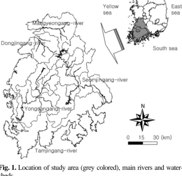
(2) 28. Gyoo-Bum Kim, Jin-Yong Lee and Kang-Kun Lee. 2. STUDY AREA The Yongsangang-Seomjingang watersheds located in the southwestern part of Korea were selected for the study because there have been many previous relevant investigations and analyses in this area (KOWACO, 1998). The total area is 18,810 km2, about 19% of South Korea, which is composed of two main watersheds, the Yongsangang and the Seomjingang, as well as other small watersheds near the South and Yellow Seas (Fig. 1). The area of the Yongsangang watershed is 3,409.2 km2 and the length of the river is about 142.7 km. In this watershed, 34.6% of the land is used for agriculture, 51.2% is forest and mountainous areas and the remaining 14.2% includes urban areas and land used for miscellaneous purposes. The surface elevation is 100−300 m, and the average topographic slope is below 2o as the region is a wide plain. The area of the Seomjingang watershed is 4,881.3 km2 and the total length of rivers is about 225.3 km. In this watershed, 18.9% of the land is used for agriculture, 72.6% is Fig. 1. Location of study area (grey colored), main rivers and waterforest and mountainous areas and the remaining 8.5% sheds. includes urban areas and land used for miscellaneous purposes. The average surface elevation is higher than that of the Yongsangang watershed and the average topographic The study area is mainly composed of 13 hydrogeologslope is also higher because of the mountainous topography ical units, which are classified based on the geologic time, and valleys that continue even into the downstream regions. rock type, hydrogeologic feature and fractures. They are The western and southern parts of the study area also have quartzite, reclaimed shore land, unconsolidated sediments, many small watersheds with smaller rivers, including the hypabyssal rock, acidic effusive rock, acidic plutonic rock, Mangyeonggang, the Dongjingang and the Tamjingang. limestone, basic plutonic rock, intermediate effusive rock, The surface elevation of these areas is below 100 m and the intermediate plutonic rock, sedimentary rock, gneiss and slopes are below 2o. schist/phyllite (Fig. 2).. Fig. 2. Regional hydrogeological unit map of Yongsangang-Seomjingang watershed..

(3) Application of representative elementary area to lineament analysis. 29. 3. METHOD AND PROCESSES 3.1. Preparing Lineament Map A lineament map was prepared using stereo photographs, which were acquired with 60% forward overlaps between successive photographs along the flight line. The photographs on a 1:20,000 scale were made several decades ago during the underdeveloped period, so that they could reflect the geologic features, faults, folds, rock types, lineaments, and topography more clearly than modern photographs. After the lineaments were extracted, we made a digital lineament map using CAD digitizers and changed it to a shape file format for ArcView analysis. Using ArcView, the number and lengths of lineaments were calculated, and then the lineaments were arranged and adjusted. We split single long lineaments into shorter lineaments automatically with ArcView script if these long lineaments were composed of two shorter lineaments with a curved external angle larger than about 200 degrees. There are a large number of lineaments in the study area (Table 1; Figs. 3 and 4). The total number of lineaments is 6,502, the total length is 21,125.7 km and the average length of a lineament is about 3.3 km. There appears no distinct specific alignment of the lineaments but lineaments with N20oE−N40oE and N30oW−N50oW are common and make up about 30% of the total. In the Yongsangang watershed, there are more lineaments than in other watersheds (the Seomjingang watershed and other small watersheds) and the lineament density is high in this watershed. Lineaments with northeast and southwest orientations are longer and more distinct along the boundary of meta-sedimentary rock and gneiss. This direction coincides with the. Fig. 3. Lineament map of Yongsangang-Seomjingang watershed.. main faults in the Cretaceous and they are the left-lateral fractures. Lineaments with east-northeast and west-southwest orientations are left-lateral fractures equal to the northeast and southwest lineaments. This direction may be the Pplane of simple shear in Riedel's model. Lineaments with north and south orientations have a relatively good continuity and a uniform distribution. This orientation coincides with the direction of extensional fractures attended by the. Table 1. (a) Basic statistics and (b) directional distribution for total lineaments of Yongsangang-Seomjingang watershed. (a) Statistics for total lineaments Number of lineaments. Total lineament length (km). Average lineament length (km). Minimum lineament length (km). Maximum lineament length (km). 6,502. 21,125.7. 3.3. 0.2. 30.9. (b) Statistics for the strike of lineaments Direction Number Percents (%) Length (km) Percents (%) Direction Number Percents (%) Length (km) Percents (%). N80W -EW 212 3.3 665.6 3.2 NS -N10E 426 6.6 1443.4 6.8. N70W -N80W 198 3.0 623.6 3.0 N10E -N20E 383 5.9 1314.1 6.2. N60W -N70W 324 5.0 923.1 4.4 N20E -N30E 485 7.5 1606.8 7.6. N50W -N60W 363 5.6 1129.3 5.3 N30E -N40E 442 6.8 1514.7 7.2. N40W -N50W 506 7.8 1669.7 7.9 N40E -N50E 352 5.4 1100.7 5.2. N30W -N40W 498 7.7 1673.1 7.9 N50E -N60E 364 5.6 1217.8 5.8. N20W -N30W 430 6.6 1352.5 6.4 N60E -N70E 326 5.0 984.0 4.7. N10W -N20W 306 4.7 919.2 4.4 N70E -N80E 260 4.0 775.4 3.7. NS -N10W 326 5.0 1102.9 5.2 N80E -EW 301 4.6 1109.8 5.3.

(4) 30. Gyoo-Bum Kim, Jin-Yong Lee and Kang-Kun Lee. Fig. 4. Orientation histogram for (a) number, (b) length and (c) average length of lineament in the Yongsangang-Seomjingang watershed.. left lateral strike-slip fractures and they are generally a normal fault. Lineaments with northwest and southeast orientations can be seen mainly in the southeastern region of the Seomjingang-Yongsangang area. These are left-lateral, weakly oblique slip and extensional lineaments. Lineaments with east and west orientations have a low frequency but a somewhat higher continuity. They are mostly extensional and are interpreted with the last stage mechanisms in this area.. 3.2. Selecting Test Points A grid system was used to obtain the data for lineament density values: the length density of lineaments, the numerical density of lineaments and the cross-points density of lineaments within the unit circular cell. The length density of lineaments is the total length (in km) of lineaments per cell area (km2), the number of lineaments is the total number of lineaments per cell area (km2) and the cross-points den-.

(5) Application of representative elementary area to lineament analysis. 31. Fig. 5. The calculation method of lineament density values using the circular method (the center of the circle is one of the grid points).. (Table 2). The smallest area of a unit circle is 0.196 km2 and the largest is 73.54 km2. After calculation of the three lineament density values for each radius, the graphs for the relation between lineament density values and radii of the unit circles were constructed, from which the REA point was determined. 3.4. Drawing the Lineament Density Map The tool used to draw the density map in this study was the Kriging Interpolater version 3.2 for ArcView Spatial Analyst, which is an extension originally developed by Marco Boeringa in September of 2001 for the hydrology department of the Amsterdam Water Supply (Gemeentewaterleidingen Amsterdam), the Netherlands. 4. REPRESENTATIVE ELEMENTARY AREA (REA) According to Hazzanizadeh and Gray (1979), REA must satisfy the inequality: Fig. 6. Actual 148 test points used to calculate the lineament density for REA analysis in Yongsangang-Seomjingang watershed.. sity is the total number of cross points of lineaments per cell area (km2) existing within the unit circular cell (Fig. 5). The test points were selected using the grid system with equal distances of 5 km latitudinally and 10 km longitudinally (Fig. 6). The total number of grid points was 148, which appeared sufficient for a statistical analysis. 3.3. Using Avenue Script in ArcView To calculate the various lineament densities, such as the lineament length density, the ArcView software from ESRI was used. Using the avenue script called PL-DENS (Program for Length DENSity calculation) developed by Kim et al. (2000), the lineament density values were computed for all 148 grid-points. The PL-DENS calculates three kinds of lineament density values: 1) lineament length density, 2) lineament crosspoints density and 3) lineament count density. To analyze the relationship between the radius of the unit circle and lineament density values, 20 different radii for the circle of 250, 500, 750, 1000, 1250, ..., 4750 and 5000 m were selected. l << D << L. (1). where l is the length scale characteristic of the rapidly varying components of the hydrologic response L, is the length scale of the slowly varying quantities, and D is the length scale of the REA. As well, the average values obtained from the target area must be independent of the size of the REA or vary only slightly with increase of its size. Lineament density maps are very important in groundwater hydrology. They can be used for groundwater investigation or management because lineaments are closely related to the presence of deep groundwater, the topography and groundwater flow mechanisms. 4.1. Lineament Length Density As shown in Table 2, the lineament length densities show diverse values that are very small or very large at a small radius such as 250 m or 500 m and are constant or change only a little at larger radii. The point where the density values become constant can be an REA for the lineament length density. If the lineament length density at a specific node point varies greatly with the variation in radius, there will be no REA. Since these increasing or decreasing length density values cause difficulties in REA interpretation, the.

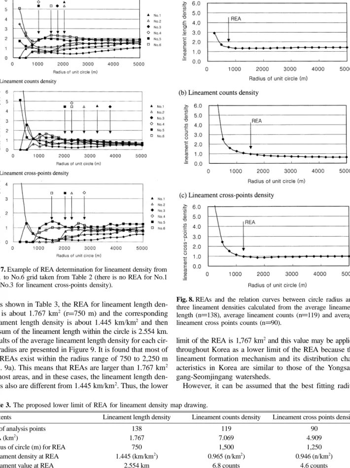
(6) 32. Gyoo-Bum Kim, Jin-Yong Lee and Kang-Kun Lee. Table 2. Results for lineament density calculation at test points for the different radius from 250 to 5,000 meters. (a) Lineament length density (unit: km/km 2) r No. 1 2 3 4 ..... 145 146 147 148. 250. 500. 750. 1000. 1250. ...... 4000. 4250. 4500. 4750. 5000. 0.000 0.000 0.000 3.468 ..... 1.965 2.310 0.000 3.391. 0.911 0.000 0.000 2.243 ..... 1.552 2.179 0.787 1.807. 1.063 0.580 0.611 1.432 ..... 1.162 1.913 0.733 1.312. 0.873 0.541 0.673 1.100 ..... 0.905 2.398 1.012 1.562. 0.738 0.511 0.612 1.136 ..... 0.861 2.167 1.142 1.641. ..... ..... ..... ..... ..... ..... ..... ..... ...... 1.312 1.527 0.834 1.485 ..... 1.073 1.374 0.890 1.405. 1.436 1.514 0.878 1.514 ..... 1.056 1.344 0.875 1.398. 1.488 1.529 0.959 1.551 ..... 1.038 1.319 0.879 1.372. 1.490 1.489 1.016 1.574 ..... 1.058 1.312 0.897 1.366. 1.495 1.444 1.071 1.612 ..... 1.053 1.295 0.915 1.342. (b) Lineament counts density (unit: n/km2) r No. 1 2 3 4 ..... 145 146 147 148. 250. 500. 750. 1000. 1250. ...... 4000. 4250. 4500. 4750. 5000. 0.000 0.000 0.000 10.186 ..... 5.093 5.093 0.000 10.186. 2.546 0.000 0.000 2.546 ..... 2.546 2.546 1.273 2.546. 1.132 0.566 1.132 1.132 ..... 1.132 2.264 0.566 1.698. 0.955 0.318 0.637 0.955 ..... 0.637 1.910 1.273 1.273. 0.815 0.611 0.407 0.815 ..... 0.611 1.222 1.222 1.019. ..... ..... ..... ..... ..... ..... ..... ..... ...... 0.577 0.676 0.458 0.458 ..... 0.378 0.557 0.458 0.497. 0.582 0.687 0.458 0.511 ..... 0.352 0.546 0.476 0.493. 0.597 0.660 0.472 0.519 ..... 0.330 0.550 0.503 0.456. 0.550 0.593 0.451 0.550 ..... 0.324 0.550 0.522 0.494. 0.535 0.547 0.446 0.547 ..... 0.318 0.522 0.497 0.446. (c) Lineament cross-points density (unit: n/km2) r No. 1 2 3 4 ..... 145 146 147 148. 250. 500. 750. 1000. 1250. ...... 4000. 4250. 4500. 4750. 5000. 0.000 0.000 0.000 0.000 ..... 0.000 0.000 0.000 5.093. 0.000 0.000 0.000 1.273 ..... 1.273 0.000 0.000 1.273. 0.000 0.000 0.000 0.566 ..... 0.566 0.000 0.000 1.132. 0.318 0.000 0.318 0.318 ..... 0.318 1.592 0.318 0.955. 0.204 0.000 0.204 0.204 ..... 0.204 1.222 0.611 0.815. ..... ..... ..... ..... ..... ..... ..... ..... ...... 0.657 0.796 0.318 0.855 ..... 0.577 0.816 0.398 0.796. 0.793 0.793 0.352 0.881 ..... 0.529 0.811 0.405 0.758. 0.833 0.865 0.456 0.880 ..... 0.487 0.817 0.456 0.692. 0.804 0.832 0.522 0.959 ..... 0.451 0.818 0.536 0.748. 0.828 0.777 0.535 1.044 ..... 0.433 0.802 0.586 0.700. values of these points (10 grid points) were discarded and only 138 data points were used. Until now, there has been a lack of adequate techniques to identify an REA. To find the inflection point, after which the length densities are constant at grid points, the curve between the circle radius and the lineament length density for each grid point was drawn (Fig. 7). While we can find the inflection point by inspection, this is somewhat artificial. A criterion for determining the best inflection point can be used: the density values should not change by 10% relative to the value for the next greater radius of the unit circle. In this study, the two important assumptions were: 1) there exists a lower limit of the REA and 2) there is a linear. regression relation between REA and lineament density values. 4.1.1. Lower limit of REA Using the method in Figure 7, the inflection points of the lineament length density for each of the 138 grid points were found. Also, the sum of the lengths of the lineaments was calculated using the lineament length density values for each grid point and the radius of the unit circle. All these lineament length values corresponding to the inflection points were arranged for each circle radius and then the average lineament length density was calculated by dividing the associated circle area (Fig. 8)..

(7) Application of representative elementary area to lineament analysis. 33. Fig. 7. Example of REA determination for lineament density from No.1 to No.6 grid taken from Table 2 (there is no REA for No.1 and No.3 for lineament cross-points density).. As shown in Table 3, the REA for lineament length density is about 1.767 km2 (r=750 m) and the corresponding lineament length density is about 1.445 km/km2 and then the sum of the lineament length within the circle is 2.554 km. Results of the average lineament length density for each circle radius are presented in Figure 9. It is found that most of the REAs exist within the radius range of 750 to 2,250 m (Fig. 9a). This means that REAs are larger than 1.767 km2 in most areas, and in these cases, the lineament length densities also are different from 1.445 km/km2. Thus, the lower. Fig. 8. REAs and the relation curves between circle radius and three lineament densities calculated from the average lineament length (n=138), average lineament counts (n=119) and average lineament cross points counts (n=90).. limit of the REA is 1,767 km2 and this value may be applied throughout Korea as a lower limit of the REA because the lineament formation mechanism and its distribution characteristics in Korea are similar to those of the Yongsangang-Seomjingang watersheds. However, it can be assumed that the best fitting radius. Table 3. The proposed lower limit of REA for lineament density map drawing. Contents No. of analysis points REA (km2) Radius of circle (m) for REA Lineament density at REA Lineament value at REA. Lineament length density. Lineament counts density. Lineament cross points density. 138 1.767 750 1.445 (km/km2) 2.554 km. 119 7.069 1,500 0.965 (n/km2) 6.8 counts. 90 4.909 1,250 0.946 (n/km2) 4.6 counts.

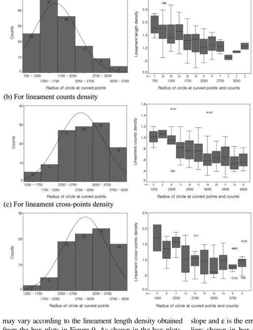
(8) 34. Gyoo-Bum Kim, Jin-Yong Lee and Kang-Kun Lee. Fig. 9. Histograms of cell radius related to the curved points and boxplots of (a) lineament length density (n=138), (b) lineament counts density (n=119) and (c) lineament crosspoints density (n=90).. may vary according to the lineament length density obtained from the box plots in Figure 9. As shown in the box plots, the median value of lineament length density and the interquartile range decrease as the radius increases. This indicates that the optimum radius for the REA is inversely proportional to the lineament length density. 4.1.2. Relation between REA and lineament length density Is the lineament-length density value useful for predicting the best fitting radius of the circle at a specific investigation area? To answer this question, a simple linear regression model was used. y = βo + β 1 x + ε. (2). where y is the radius of circle, x is the lineament length density value, βo is the intercept of the line of best fit, β1 is its. slope and ε is the error term. During the regression, the outliers shown in box-plots in Figure 9 were excluded. The number of outliers is 1 for lineament length density value, 3 for lineament counts density and 6 for lineament crosspoints density. Tables 4 and 5 are the results of linear regression model analyses for the relationships between circle radius and each of lineament length density, lineament counts density and lineament cross-points density. The value of R, the simple correlation between lineament length density and the radius of the circle, is 0.487. The coefficient of determination, R2, is 0.237 and explains 23.7% of the variance of the circle radius. However, the F-statistic, 41.0 and p-value, 0.0, indicate that the slope, β1, is not zero and the linear relation is highly significant. Estimates of the model coefficients, βo (intercept) and β1 (slope) are 2,545.7 and −602.6, respectively. So the estimated linear regression model for the lineament length density is:.

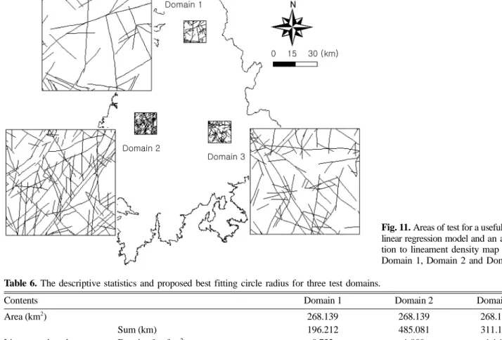
(9) Application of representative elementary area to lineament analysis. 35. Table 4. Descriptive statistics for lineament density computed with each REA corresponding to diverse circle radius at the test points of Yongsangang-Seomjingang watershed. Contents Lineament length density Lineament counts density Lineament cross-points density. n. Mean of density. S.D. of density. Minimum density. Maximum density. 137 116 184. 1.402 0.714 1.000. 0.500 0.221 0.421. 0.23 0.29 0.25. 2.67 1.21 2.12. Table 5. Result of linear regression model analysis to examine the relation between lineament density and circle area. (a) Model summary Model Lineament length density Lineament counts density Lineament cross-points density. R 0.487 0.522 0.423. R Square 0.237 0.273 0.179. Adjusted R Square 0.232 0.266 0.169. Std. Error of the Estimate 541.89 556.86 561.52. Durbin-Watson 2.195 2.160 1.899. (b) ANOVA Model Lineament length density Lineament counts density Lineament cross-points density. Sum of squares 12,337,512 13,250,541 15,642,065. Degree of freedom 1 1 1. Mean Square 12,337,512 13,250,541 15,642,065. F-statistic 41.015 42.731 17.894. Sig. level 0.000 0.000 0.000. (c) Coefficients Model. Contents. Lineament length density. Constant Radius of circle Constant Radius of circle Constant Radius of circle. Lineament counts density Lineament cross-points density. Unstandardized coefficients Standardized coefficients B 2,545.7 -602.6 4,026.8 -1,538.4 -3,613.4 1,,-619.3. Std. Error 138.335 192.969 175.737 235.343 158.714 146.412. β -0.487 -0.522 -0.423. t-statistic. Sig. level. 18.402 -6.482 22.914 -6.537 22.767 -4.230. 0.000 0.000 0.000 0.000 0.000 0.000. (d) Residual statistics and diagnostics Model Lineament length density Lineament counts density Lineament cross-points density. Standardized residual (minimum) -2.159 -2.735 -2.359. Standardized residual (maximum) 3.087* 2.205* 1.895*. Radius of circle=2,545.7−602.6×Total lineament length density (3) Also, the t-statistic and p-value indicate that the slope of this model is significant. Scatter plots for the standardized predicted value and radius are presented in Figure 10. The minimum and maximum standardized residuals are −2.159 and 3.087, respectively, and most of residuals fall between −2 and +2 (only 1 in 137 fall outside +3). From the normal p-p plot and the normal distribution of the standardized residuals, the residuals follow a normal distribution because the plotted values fall mostly along the line (Fig. 10). This shows that this model can be generally accepted. In the scatter plots for. VIF. Remarks. 1.000 1.000 1.000. *There is only one data larger than 3 in standard residual value. standardized predicted value and the circle radius, the predicted values show a slight directional feature along the straight line extending from the lower left corner to the upper right so this model cannot be rejected. From the regression results, it is likely that the lineament length density could be related to the radius of the circle although the coefficient of determination appears low. The above linear regression model was applied to three test areas to reveal that different radii should be used for areas with a different lineament length density (Fig. 11). The descriptive statistics for the three areas are presented in Tables 4, 5 and 6. As shown in Table 6, the three domains have different areas and different lineament density values. Domain 2 has the largest lineament-length density value,.

(10) 36. Gyoo-Bum Kim, Jin-Yong Lee and Kang-Kun Lee. Fig. 10. Standardized residual histograms and Normal P-P plots.. 1.809 km/km2, and Domain 1 has the smallest, 0.732 km/km2. If the regression model is correct and useful, we can apply different REA to each domain because they have different lineament density values. This means that the lineament density map drawn with the density values calculated from the best fitting radius (REA) is acceptable to represent lineament distribution patterns. We selected the radii r1, r2 and r3 (r1<r2<r3) and here r2, a proposed value in Table 6, is the best fitting size (2,105 m for Domain 1, 1,456 m for Domain 2 and 1,846 m for Domain 3) of the radius calculated from the regression model. For testing the model fitness, r1, 1,000 m smaller and r3, 1,000 m larger than r2 were selected. Nine linea-. ment-length density maps from lineament maps for the three domains are drawn for the three radii, r1, r2, and r3 (Fig. 12). In drawing the density maps, we used the ordinary kriging method in Kriging Interpolater version 3.2 for ArcView Spatial Analyst, in which the semi-variogram is fit to the variance points using the Levenberg-Marquardt method of nonlinear least squares approximation. To measure the goodness of fit of the semi-variogram, AIC (Akaike Information Criteria), BIC (Bayesian Information Criteria) and SSE (The Sum of the Square of the weighted differences) were used. As shown in the three domains in Figure 12, the domain with a larger lineament density has a smaller radius of circle. For each domain, the density map made with the small-.

(11) Application of representative elementary area to lineament analysis. 37. Fig. 11. Areas of test for a usefulness of linear regression model and an application to lineament density map for Domain 1, Domain 2 and Domain 3. Table 6. The descriptive statistics and proposed best fitting circle radius for three test domains. Contents 2. Area (km ) Lineament length. Lineament counts. Lineament cross-points. Sum (km) Density (km/km2) Proposed best radius of circle (m) Sum (n) Density (n/km2) Proposed best radius of circle (m) Sum (n) Density (n/km2) Proposed best radius of circle (m). est radius looks adequate, but in this case, most of the highdensity classes are shown near the lineament itself or lineament intersections with a very narrow range. This density map may not be adequate to analyze the relation between lineament density and groundwater productivity or well yield. The density map with the largest radius looks inadequate because most lines of equal density intersect and penetrate the lineaments and the lineament density classes cannot represent properly the lineament-length density distribution. Therefore, the lineament density maps produced with the circle radius from the linear regression model, the second map of the three domains in Figure 12, can illustrate the characteristics of lineament distribution thoroughly. 4.2. Lineament Counts Density Like lineament length density, the number of lineaments. Domain 1. Domain 2. Domain 3. 268.139 196.212 0.732 2,105 58 0.216 3,694 62 0.231 3,470. 268.139 485.081 1.809 1,456 177 0.660 3,011 379 1.413 2,738. 268.139 311.163 1.160 1,846 108 0.403 3,407 184 0.686 3,188. within the circle (unit: number/km2) along the grid points was calculated (see Table 2). At each grid point, the best circle size for the inflection point was determined using the 10% rule. Additionally, we did not consider the lineament counts densities that did not show 10% or less variation. Therefore, the number of points tested was only 116 points, except for the outliers. Using the same method as for the lineament length density, the minimum REA for lineament counts density was determined as about 7.069 km2 (1,500 m radius), which is much larger than the lineament length. The corresponding lineament counts density is about 0.965 and the sum of its numbers within the circle is 6.8 (see Table 3 and Fig. 8). From the histogram (b) in Figure 9, it is observed that most of the REAs exist within the range from 2,250 to 3,750 m. Also, the box-plots indicate that REAs vary only slightly with changes in the lineament counts density. The mean of the lineament counts density decreases with the.

(12) 38. Gyoo-Bum Kim, Jin-Yong Lee and Kang-Kun Lee. Fig. 12. Lineament length density maps drawn for three radii using the result of PL-DENS in the three domains.. increase of the radius. Using the relationship between each REA and the lineament counts density for all points, we can find the representative REA. Based on a simple linear regression model (Tables 4 and 5), the regression equation (4) was considered to account for the REA.. Radius of circle=4,026.8−1538.4×Total lineament counts density (4) Based on the residual statistics, normal probability plotting and the scatter plot for standardized predicted value.

(13) Application of representative elementary area to lineament analysis. 39. Fig. 13. Lineament counts density maps drawn for three radii using the result of PL-DENS in the three domains.. and the circle radius, this model can be accepted even though the coefficient of determination is low. To apply this model to the three domains as for the lineament length density analysis, we calculated the best fitting circle radius for each domain: 3,694 m for Domain 1,. 3,011 m for Domain 2 and 3,407 m for Domain 3 (Table 6). Next, the lineament counts density maps for three radius, r1, r2 and r3 for each domain were drawn (Fig. 13). As shown in the figure, different radii can be applied according to the size of the lineament counts density. The optimum circle.

(14) 40. Gyoo-Bum Kim, Jin-Yong Lee and Kang-Kun Lee. Fig. 14. Lineament cross-points density maps drawn for three radii using the result of PL-DENS in the three domains.. radius, which is obtained from the regression model, is adequate, based on nine lineament density maps of the three domains. But, as shown in Figure 9, the lineament counts density values, which correspond to radii from 2,250 to. 2,750 m, do not have unique trends but are similar. This means that the REA cannot show a distinct variation for this range of radii and we should be careful in applying this regression result..

(15) Application of representative elementary area to lineament analysis. 41. 4.3. Lineament Cross-Points Density. 5. SUMMARY AND CONCLUSIONS. Lineament cross-points are important for groundwater exploration and deep groundwater development. Using the lineament map, we calculated the number of lineament cross-points within the circle along the 148 grid points (see Table 2). At each grid point, the best circle size for the inflection point using the 10% rule was found as for the lineament length density. Also, the continuously increasing or decreasing counts densities were not considered and so the number of testing points equals 84, except for six outliers. The REA for lineament cross-points density is about 4.909 km2 (r=1,250 m) and the corresponding lineament cross-points density is about 0.946/km2, which means the count sum is 4.6 (see Table 3 and Fig. 8). From the histogram (c) in Figure 9, it is seen that most of the REAs exist within the range of 2,250 to 3,750 m. Also, the box-plots show that the REA varies with the lineament cross-points density. The mean value of lineament cross-points density decreases gradually with the increasing of the radius. From the relationship between REA and lineament crosspoints density, we can find the best REA. The simple linear regression Eq. (5) was considered.. The lower limits of the REA of the study area are about 1.767 km2 (r=750 m) for drawing lineament-length density maps, 7.069 km2 (r=1,500 m) for drawing lineament counts density maps and 4.909 km2 (r=1,250 m) for drawing lineament cross-points density maps. From analyses of the relationship between circle radii (REAs) and lineament density values, it is found that the radius (REA) is inversely proportional to the lineament density, which was demonstrated by the linear regression model tests. When we draw the lineament-length density map and the lineament-counts density map, we should calculate the lineament density values for the whole area and then find the REA (or the best circle radius) using a linear regression model. However, lineament cross-points density values should be carefully calculated because the determination coefficient of the linear regression model is very low. Also, the same attention should be paid to calculation of the lineament counts density values, because the REA cannot have an obvious effect upon the results of the density calculation from 2,250 m to 2,750 m of circle radius. Because extraction of the lineament from remote sensing data is generally done with a 1/25,000 scale in Korea, the results of this study done with the lineament map of 1/25,000 can be used usefully and practically. To date, lineament density maps, including lineament-length density and crosspoints density maps, have been drawn with an arbitrary circle radius. However, the circle radius for drawing the lineament density maps can be carefully selected by applying the linear regression models suggested in this study. The limitation of this study is that the study area, the Yongsangang-Seomjingang watershed, has so many lineaments, which are relatively evenly distributed in diverse directions produced by many complicated geologic events and history. If many lineaments are arranged along the predominant direction, the linear regression model of this study for the calculation of lineament density values may need to be amended. If there are some directional distributions of lineaments, it is expected that the lineament length density may be larger, but the number of lineament crosspoint in the unit circle may be much less than the value, which is made from linear regression model in this study.. Radius of circle=3,613.4−619.3×Total lineament cross points density (5) This model can be accepted based on the residual statistics, normal probability plotting and scatter plots for the standardized predicted value and the circle radius, even if the coefficient of determination is very low. To apply this model to the three domains, we calculated the best fitting radius of the circle for each domain: 3,470 m for Domain 1, 2,738 m for Domain 2 and 3,188 m for Domain 3 (Table 6). Next, the lineament cross-points density maps for 3 radii, r1, r2 and r3 were drawn (Fig. 14). As shown in Figure 14, however, it is not easy to distinguish the difference between the lineament density maps based on the smallest radius and the proposed best radius from a regression model for the three domains. That is to say, because the coefficient of determination, R2=0.179, is too low, the regression model determining the circle radius for the lineament cross-points density calculation should be applied carefully to these domains. The lineament cross points density map made with the smallest radius (r1) shows that the intervals between the lines of equal density is not uniform. Therefore, these maps appear not fit to analyze the relation between the lineament density and groundwater characteristics. Consequently, for the lineament cross-points density map, the most effective map is the map made by the circle radius of REA. When we draw a lineament crosspoints density map, in particular, the effectiveness of the circle radius should be considered because of the low determination coefficient.. ACKNOWLEDGMENTS: This work was partly supported by Korea Research Foundation (#DS0072) through the third author.. REFERENCES Bear, J., 1972, Dynamics of fluids in porous media. Elsevier, New York, 764p. Caponera, F., 1989, Remote sensing applications to water resources: remote sensing image interpretation for ground water surveying. Food and Agriculture Organization of the United Nations, Rome, 393 p..

(16) 42. Gyoo-Bum Kim, Jin-Yong Lee and Kang-Kun Lee. Casas, A.M., Cortes, A.L., Maestro, A., Soriano, M.A., Riaguas, A. and Bernal, J., 2000, LINDENS: a program for lineament length and density analysis. Computer Geosciences, 26, 1011−1022. Costa, R.D. and Starkey, J., 2001, Photolin: a program to identify and analyze linear structures in aerial photographs, satellite images and maps. Computer Geosciences, 27, 527−534. ESRI (Environmental Systems Research Institute, Inc.), 1996, Using Avenue: customization and application development for ArcView GIS. ESRI, Redlands, CA, 340 p. Hazzanizadeh, M. and Gray, W.G., 1979, General averaging equations for multi-phase systems: 1. Averaging procedure. Adv. Water Res., 2, 131−144. Hobbs, B.E., Means, W.D. and Williams, P.F., 1976, An outline of structural geology. John Wiley & Sons, New York, p. 571. Karnieli, A., Meisels, A., Fisher, L. and Arkin, Y., 1996, Automatic extraction and evaluation of geological linear features from digital remote sensing data using a Hough transform. Photogrammetric Engrg Remote Sensing, 62, 525−531. Kim, C., 1995, GIS application to groundwater study. Kor. Soc. J. Civil Engineers, 15, 149−156. Kim, G.B., 1999, Guideline for construction and management of hydrogeological map in Korea. Journal of Korean Water Research, 32, 82−95. Kim, G.B., Cho, M.J. and Lee, J.Y., 2000, A study on the illustration of hydrogeological map using ArcView and AvenueTM script. In Proceedings of 2000 Fall Meeting of Korean Society of Soil and Groundwater Environment (Abstract). Pohang, November, 17−18, p. 31−35. Koike, K., Nagano, S. and Ohmi, M., 1995, Lineament analysis of satellite images using a segment tracing algorithm (STA). Computer Geosciences, 21, 1091−1104. KOWACO (Korea Water Resources Corporation), 1998, Hydrogeo-. logical survey of Yongsangang-Seomjingang watersheds. Lattman, L.H. and Parizek, R.R., 1964, Relationship between fracture traces and the occurrence of ground water in carbonate rocks. Journal of Hydrology, 2, 73−91. Mabee, S.B., Hardcastle, K.C. and Wise, D.U., 1994, A method of collecting and analyzing lineaments for regional-scale fracturedbedrock aquifer studies. Ground Water, 32, 884−894. Magowe, M. and Carr. J.R., 1999, Relationship between lineaments and ground water occurrence in western Botswana. Ground Water, 37, 282−286. Mah, A., Taylor, G.R., Lennox, P. and Ballia, L., 1995, Lineament analysis of Landsat thematic mapper images, Northern Territory, Australia. Photogrammetric Engrg Remote Sensing, 61, 761−773. O’Leary, D.W., Freidman, J.D. and Pohn, H.A., 1976, Lineaments, linear, lineation-some proposed new standards for old terms. Geological Society of America Bulletin, 87, 1463−1469. Park, Y.J., Lee, K.K. and Kim, J.M., 2000, Effects of highly permeable geological discontinuities upon groundwater productivity and well yield. Mathematical Geology, 32, 605−618. Razavi, A.H., 1995, ArcView developer's guide. OnWord Press, New York, 274 p. Saraf, A.K., 2001, Drainage/lineament/roads density analyst extension (version 1.0). ESRI, Redlands, CA. Wood, E.F., Sivapalan, M., Beven, K. and Band, L., 1988, Effects of spatial variability and scale with implications to hydrologic modeling. Journal of Hydrology, 102, 29−47. Yin, Z.Y. and Brook, G.A., 1992, The topographic approach to locating high-yield wells in crystalline rocks: does it work? Ground Water, 30, 96−102. Manuscript received December 13, 2003 Manuscript accepted February 11, 2004.

(17)