Evaluating Applicability of Sediment Transport Capacity Equations through Sensitivity Analysis
민감도 분석을 통한 유사이송용량 산정식의 적용성 평가
Her, Younggu*・ Hwang, Syewoon**,†
허용구 ・ 황세운
Abstract
유사는 오염물질을 저장 또는 운반하는 매개체로 하류 수체의 물리적, 화학적, 생물학적 과정에 큰 영향을 미친다. 따라서 유사 발생 및 운송 양의 추정은 수질개선을 위한 유역관리계획을 수립하는데 중요한 자료가 된다. 이러한 유사량 및 운송과정은 주로 모형에 의해 계산되고 모의되는데, 많은 유사운송모형들이 유사이송용량 (sediment transport capacity)식을 이용하여 유사 발생량, 이송량 및 퇴적량을 산정한다. 유출에 의한 유사이송용량을 산정하기 위한 기존의 식들은 각기 다른 목적과 환경에서 개발 되어 보편적으로 적용할 수 있는 식은 전무한 실정이다. 이에 본 연구는 유사이송용량을 계산하기 위해 사용되는 식들의 개발 목적과 환경을 검토하고, 경사, 유량, 유사입경 및 토성에 따른 민감도를 조사하여 각 식의 적용성을 평가하였다. 본 연구에서 적용한 8개의 유사이송용량 산정식은 모두 경사도에 가장 민감하게 변화하는 것으로 나타났 다. Abraham과 Yalin식 이외의 산정식을 이용하여 계산된 유사이송용량은 경사도가 0.1 % 보다 작을 때는 0 mg/l, 경사도가 100 % 보다 클 때는 이론최대치인 2,650 mg/l 을 넘는 것으로 나타나, 이들 산정식의 적용 가능한 경사도 범위를 0.1 %-100 %로 추정할 수 있었다. Abrahams식은 유량에, Bagnold식은 유사입경 및 토성에 민 감한 것으로 나타났다. Low, Rickenmann, 및 Schoklitsch식은 유량에 민감하게 반응하지 않았고, Low와 Schoklitsch식은 토성에도 민감하지 않은 것으로 나타나, 이 들 식의 제한된 적용성을 확인하였다. 한편, Yang식은 계산식에 포함된 로그항으로 인해 그 적용범위가 제한되는 경우가 있었다. Abrahams과 Yalin식을 이용하여 산정 된 유사운송용량은 모든 인자들에 민감하게 반응하는 것으로 나타났으며, Yalin과 Low식의 경우, silt와 clay에 적용되었을 때 유량이 클수록 유사운송용량이 다소 작아 지는 경향을 보임에 따라, 전체적으로 Abraham식의 적용성이 가장 높은 것으로 평가되었다. 본 연구결과는 향후 모형을 이용한 유사량 모의 시 적용대상 지역의 특성에 가장 적합한 유사운송용량 산정식을 선정하는데 유용한 정보를 제공할 것으로 기대된다.
Keywords: sediment transport capacity; sensitivity analysis; slope; discharge; soil texture; characteristic sediment particle size
* Blackland Research Center, Texas A&M University, Temple. TX, USA
** Dept. of Agricultural eng., (Institute of Agriculture and Life Science), Gyeongsang Nat. Univ., Jinju, Korea
† Corresponding author
Tel.: +82-55-772-1934 Fax: +82-55-772-1939 E-mail: [email protected]
Received: August 4, 2015 Revised: October 29, 2015 Accepted: November 2, 2015
Ⅰ. INTRODUCTION
Sediments originate from soil and other suspended matter carried in flowing water, or they are formed within a waterbody itself as a result of growth, metabolism, and death of plants and animals. Sediment is not only the major pollutant by weight and volume but it also serves as a catalyst, carrier, and storage agent of other forms of pollution (ASCE, 2006). Thus, physical, chemical, and biological processes occurring in a waterbody are significantly influenced by sediments (DiToro, 2001). Sediment together with pathogens
and habitat alterations were cited as the leading causes of impairment in rivers and streams of the USA (EPA, 2007).
Sediments may reduce visibility, shorten the depth of the photic zone, and then alter the vertical stratification of heat in the water column by suspending in a waterbody (Wilber et al., 2001). In addition, sediment may lead to capacity loss of reservoir, channel, and wetland and efficiency loss of man-made structure such as intake of a dam and irrigation canal by filling their storage and blocking path (Morris et al., 1998). At the same time, however, nutrients, detritus, and other organic matter transported with sediment particles are critical to the health of a waterbody (EPA, 2003). Sediment in natural quantities also replenishes sediment bedloads and creates micro-habitats such as pools and sand bars (EPA, 2003). In general, sediment may be considered a pollutant when it exceeds natural concentration and has a detrimental effect on water quality in a biologic and/or esthetic sense (Dunne et al., 2002). On the other hand, clear water with little sediment and high flow energy can cause excessive
scour on the waterbody boundary such as streambed degra- dation, bank failure, channel armoring, and degradation of stream habitat (Morris et al., 1998). Thus, accurate estimation of sediment loads should be necessary in developing watershed management plans to improve the environmental quality and health of a waterbody.
There are two main approaches in simulating mechanisms of sediment transport: supply-limited and capacity-limited.
In the supply-limited approach, sediment transport is limited by the upstream supply of sediments (Julien, 1995), and transportation capacity is assumed to be unlimited. USLE (Universal Soil Loss Equation) is a typical for supply- limited approach (Kang et al., 2003; Her et al., 2006; Lee et al., 2006; Song and Lim, 2014). The amount of sediment that can be supplied is closely related to the characteristics of bed soil, and it is usually estimated by measuring physical parameters such as shear stress or soil erodibility. On the other hand, the capacity-limited approach assumes that sediment transport is controlled by carrying capacity of flow, and sediment is supplied sufficiently or unlimitedly.
The sediment transport capacity concept is a type of this approach. The transport capacity is associated with the characteristics of flow and sediment such as flow energy, sediment particle size, and concentration.
In the reality, the two approaches may control sediment transport reciprocally so that one approach alone may be not enough to explain sediment transport phenomena completely except for some extreme cases such as completely armored channel (supply-limited) and hyperconcentrated flow (capacity- limited). In general, however, capacity-limited and supply- limited conditions are assumed dominant on highly and less erodible soils, respectively (Haan et al., 1994). Shear stress of overland flow is low due to small flow discharge rate per unit width even though slope of the overland area is usually much steeper than that of a stream, so thus transport capacity of overland flow is likely to be smaller than that of channel flow. In addition, the shallow depth of overland flow may limit some sediment transport mechanisms such as suspension and saltation (Julien et al., 1985). Thus, bedload may pre- dominate in the overland flow, and its movement is largely controlled by the transport capacity of the flow (Julien et al., 1985; Haan et al., 1994). On the other hand, it is often assumed that washload travels by stream flow with little
deposition, and it is carried primarily in suspension (Haan et al., 1994). Thus, total sediment load of the stream flow consists of bedload and washload. In general, the finer sediment particle has less availability in the watershed (Haan et al., 1994). Fine sediment particles may show high spatial variability because they are detached and transported relatively easily due to lightweight and deposited in a calm waterbody having slow flow velocity. Therefore, trans- portation of washload or suspended sediment is subject to be limited by supply of fine sediment.
Many sediment transport simulation models adapt both approaches Meyer and Wischmeier (1969) proposed and Foster and Meyer (1972) proposed to determine transport processes (detachment and deposition) and estimate rates of them. Various types and forms of the transport capacity relations are used in physically based sediment transport model such as CREAMS (Silburn and Loch, 1989), WEPP (Foster et al., 1995), KINEROS (Woolhiser et al., 1990), ANSWERS (Beasley and Huggins, 1981), AGNPS (Young et al., 1989), GUESS (Misra and Rose, 1996), EUROSEM (Morgan et al., 1998), and LISEM (Jetten, 2002). One of the widely used equations for estimating the transport capacity is the Yalin sediment transport equation. CREAMS, WEPP, and ANSWERS adapt modifications of the Yalin equation.
The equation compares the critical shear stress with shear stress of flow acting on the bed. In AGNPS and GUESS, the transport capacity is estimated by the stream power concept of Bagnold (1966) and its variation, which emphasizes energy (potential) of flow rather than force or stress being applied to the bed. The stream power per unit area of bed is calculated by multiplying specific weight of water, discharge per unit width, and local energy gradient (or surface slope) together. In addition, the transport capacity is modeled as a function of the unit stream power Yang (1973) and Govers (1990) proposed in KINEROS, EUROSEM, and LISEM. The unit stream power is calculated by multiplying mean velocity of flow by local energy gradient.
There are many equations proposed to calculate the sediment transport capacity based on sediment flow hydraulics, topography, and soil characteristics. Each equation has its own applicable range corresponding to the environment for which it was developed. The range of applicable slopes, targeted sediment types, and available
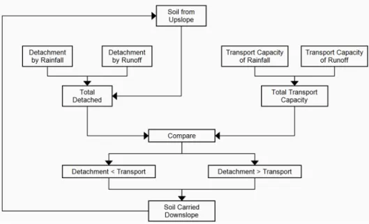
Fig. 1 Transport capacity in a capacity-limted approach (Meyer and Wischmeier, 1969; Her, 2011) data for application of the equations would be crucial
considerations in choosing an equation for sediment transport modeling. However, our understandings on the application ranges of the equations are not sufficient to help select appropriate transport capacity equations in sediment modeling. This study investigated how sediment transport capacity calculated using eight different equations commonly employed in sediment modeling responds to changes in flow discharge, slope, characteristic sediment particle size, and soil texture. In addition, their development environments were surveyed from literature where the equations were introduced. Understanding their sensitivity to the potential application conditions is expected to provide information useful in selecting equations for calculating sediment transport capacity in sediment modeling.
Ⅱ. METHOD AND MATERIAL
1. Sediment Transport Capacity Concept
Many sediment transport models adapted the concept Meyer and Wischmeier (1969) proposed based on the capacity-limited approach in order to calculate detachment or deposition rate of sediment. In the concept, the estimated transport capacity is used to determine which sediment transport process of between detachment and deposition
would occur and its rate in the given condition (Fig. 1).
Foster and Meyer (1972) proposed a continuity equation for describing mass balance of sediment transport processes occurring on interrill and in rill. The basic form of the equation is like below.
(1)
where is sediment load, is a delivery rate of sediment detached on interrill to rill, is a rate of detachment or deposition of sediment in rill flow. Foster and Meyer (1972) also expressed a continuity equation of sediment transport as a relationship between sediment detachment and deposition like below.
(2)
where is detachment rate, is detachment capacity,
is sediment load, and is transport capacity. In this relationship, "when hydraulic shear stress exceeds the critical shear stress of the soil and when sediment load is less than sediment transport capacity, net soil detachment in rills is calculated“ using the following equation (Nearing et al., 1989):
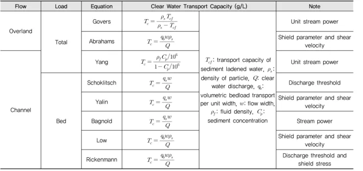
Table 1 Equations for calculating sediment transport capacity (revised from Hessel et al., 2007)
Flow Load Equation Clear Water Transport Capacity (g/L) Note
Overland
Total
Govers
: transport capacity of sediment ladened water, : density of particle, : clear
water discharge, : volumetric bedload transport per unit width, : flow width,
: fluid density, : sediment concentration
Unit stream power
Abrahams
Shield parameter and shear
velocity
Channel
Yang
Unit stream power
Bed
Schoklitsch
Discharge threshold
Yalin
Shield parameter and shear
velocity
Bagnold
Stream power
Low
Shield parameter and shear
velocity
Rickenmann
Discharge threshold and
shield stress
(3)
“When hydraulic shear stress exceeds critical shear stress for the soil, detachment capacity" is calculated using Eq. (4) (Nearing et al., 1989).
(4)
where is channel soil erodibility, is flow shear stress, is critical shear stress of a soil. Finally, the detachment rate equation will become Eq. (5), so thus the approach can consider both supply-limited and capacity- limited cases with transport capacity and cases with channel soil erodibility, respectively.
(5)
Julien et al. (1985) proposed a general form of the equations for calculating the sediment transport capacity of overland flow (Eq. (6)).
(6)
where , , , and are coefficients determined empirically.
2. Sediment Transport Capacity Equation
There are many equations proposed to estimate sediment transport capacity of flow, and this study focused eight equations commonly used in sediment transport simulations, which were restated by Hessel et al. (2007) (Table 1):
Govers, Abrahams, Yang, Schoklisch, Yalin, Bagnold, Low, and Rickenmann equations (Schoklitsch, 1962; Yalin, 1963;
Yang, 1973; Bagnold, 1980; Low, 1989; Rickenmann, 1991;
Govers, 1990; Guy et al., 1992; Abrahams et al., 2001; US Department of the Interior, 2006; Hessel et al., 2007). As seen in Table 1, the Govers and Abrahams equations were originally developed for estimating total sediment transport capacity of overland flow, but the others were proposed for calculating bedloads of channel flow, except for the Yang equation developed for calculating total sediment loads of channel flow. The equations were formulated based on their own concepts of sediment detachment and transport mechanisms, which make them unique in terms of equation forms and application ranges. Details of the equations can be found in Hessel et al. (2007), and only their important characteristics are summarized here.
3. Pedotransfer Function for Characteristic Sediment Particle Sizes
Calculation of sediment transport capacity requires information of characteristic sediment particle sizes (D50, D40, D30, and D90). However, there is no known soil database that provides a particle-size distribution of a soil, and it is not efficient to conduct sieving tests with sampled soils. Thus, in this study, a pedotransfer function (Eq. 7) proposed by Skaggs et al. (2001) was utilized to develop particle-size distributions for soils in estimating the characteristic sediment particle sizes (Fooladmand and Sepaskhah, 2006).
exp
(7)
where is radius of sediment particle, is the mass fraction of sediment particle less than the radius , is the fraction of clay, and is parameters.
(8)
ln (9)
ln (10)
ln (11)
ln (12)
ln (13)
where is the fraction of silt, is the fraction of fine and very fine sands.
4. Sensitivity Analysis
Sensitivity of sediment concentrations calculated using sediment transport capacity equations to slopes, flow dis-
charges, characteristics sediment particle sizes, and soil textures was investigated to assess their applicability in terms of soil characteristics, topography, flow types (overland and channel flow) with consideration of their development environments surveyed from the original literature (Table 2). For this sensitivity analysis, the Manning's roughness coefficient and channel width were set to 0.03 s/m1/3 and 30 m, respectively, while slope, flow discharge, particle size, and soil texture vary within predefined ranges. Then, flow depth was calculated through an iterative solution of Manning’s equation with flow discharge given, roughness coefficient, and slope. The settling velocity of a sediment particle was calculated using Stokes’ law assuming the particle density of 2.65 g/cm3 and the flow temperature of 20
°C in which dynamic viscosity can be approximated to 0.001 kg/m/s. For simplicity of the analysis, characteristic sediment particle sizes for D50 were assumed as 0.75 mm, 0.05 mm, and 0.002 mm for sand, silt, and clay, respectively, according to the USDA soil classification (USDA, 1987).
Ⅲ. RESULTS AND DISCUSSION
1. Development Environments of Transport Capacity Equations
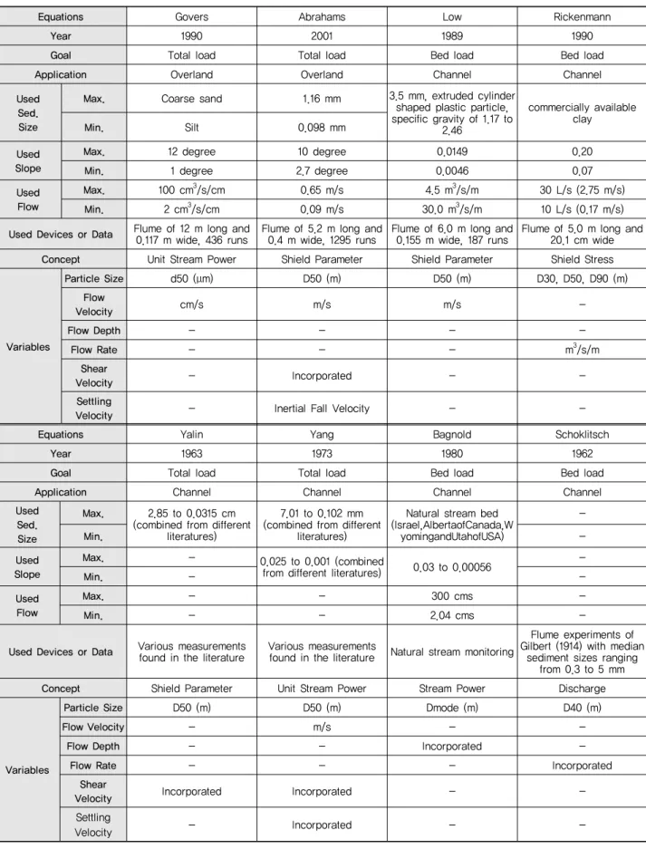
Features of the equations including the environment for which they were developed, sediment types, and concepts were investigated from literature, and they are summarized in Table 2. The Yalin and Yang equations were driven based on measurements found in literature. The Yalin equation was recommend in estimating transport capacity for shallow overland and channel flow, and Foster and Meyer (1972) concluded that the Yalin equation was most appropriate for shallow flows associated with upland erosion (Meyer Wischmeier, 1969; Alonso et al., 1981; Frinkner et al., 1989). On the other hand, the slope ranges, 1 to 12 degree, used for developing the Govers and Abrahams equations indicate that they can be better applied to overland flow rather than channel flow, and thus they are reasonably expected to provide significant underestimation on sediment transport capacity of channel flow. Although a general approach to sediment transport simulation for overland flow is usually applicable to channel flow, selections of the transport capacity relation can be different for the two flow
Table 2 Development environment of the sediment transport capacity equations
Equations Govers Abrahams Low Rickenmann
Year 1990 2001 1989 1990
Goal Total load Total load Bed load Bed load
Application Overland Overland Channel Channel
Used Sed.Size
Max. Coarse sand 1.16 mm 3.5 mm, extruded cylinder
shaped plastic particle, specific gravity of 1.17 to
2.46
commercially available
Min. Silt 0.098 mm clay
SlopeUsed
Max. 12 degree 10 degree 0.0149 0.20
Min. 1 degree 2.7 degree 0.0046 0.07
Used Flow
Max. 100 cm3/s/cm 0.65 m/s 4.5 m3/s/m 30 L/s (2.75 m/s)
Min. 2 cm3/s/cm 0.09 m/s 30.0 m3/s/m 10 L/s (0.17 m/s)
Used Devices or Data Flume of 12 m long and
0.117 m wide, 436 runs Flume of 5.2 m long and
0.4 m wide, 1295 runs Flume of 6.0 m long and
0.155 m wide, 187 runs Flume of 5.0 m long and 20.1 cm wide Concept Unit Stream Power Shield Parameter Shield Parameter Shield Stress
Variables
Particle Size d50 (μm) D50 (m) D50 (m) D30, D50, D90 (m)
Flow
Velocity cm/s m/s m/s -
Flow Depth - - - -
Flow Rate - - - m3/s/m
Shear
Velocity - Incorporated - -
Settling
Velocity - Inertial Fall Velocity - -
Equations Yalin Yang Bagnold Schoklitsch
Year 1963 1973 1980 1962
Goal Total load Total load Bed load Bed load
Application Channel Channel Channel Channel
UsedSed.
Size
Max. 2.85 to 0.0315 cm (combined from different
literatures)
7.01 to 0.102 mm (combined from different
literatures)
Natural stream bed (Israel,AlbertaofCanada,W
yomingandUtahofUSA)
-
Min. -
Used Slope
Max. - 0.025 to 0.001 (combined
from different literatures) 0.03 to 0.00056 -
Min. - -
UsedFlow
Max. - - 300 cms -
Min. - - 2.04 cms -
Used Devices or Data Various measurements
found in the literature Various measurements
found in the literature Natural stream monitoring
Flume experiments of Gilbert (1914) with median
sediment sizes ranging from 0.3 to 5 mm
Concept Shield Parameter Unit Stream Power Stream Power Discharge
Variables
Particle Size D50 (m) D50 (m) Dmode (m) D40 (m)
Flow Velocity - m/s - -
Flow Depth - - Incorporated -
Flow Rate - - - Incorporated
Shear
Velocity Incorporated Incorporated - -
Settling
Velocity - Incorporated - -
conditions (Woolhiser et al., 1990). Some of the equations were developed based on flume experiments (the Govers, Abrahams, Low, Rickenmann, and Schoklitsch equations) and monitoring data from natural streams in three specific regions (Israel, Alberta, and Utah: Bagnold’s equation), thus their application ranges could be limited. Moreover, the use of artificial particles in a specific shape may further limit the application ranges of the Low and Rickenmann equations.
The unit stream power concept defined as “the time rate of potential energy expenditure per unit weight of flow“ was adapted in the Govers and Yang equations (Yang and Stall, 1974). The Bagnold equation uses the stream power concept that is slightly different from the stream power concept, which is defined as a rate of energy dissipation to the stream beds (Bagnold, 1980). On the other hand, the Abrahams, Low, Yaling, and Rickenmann equations employ the Shields parameter or Shields stress to define incipient motion of a sediment particle. All equations investigated in this study are commonly based on the incipient motion concept assuming a threshold condition that initiates movement of a single soil grain and requires information of characteristic diameter (or radius), such as D50, D30, and D90, as the representative feature of sediment particles to be simulated.
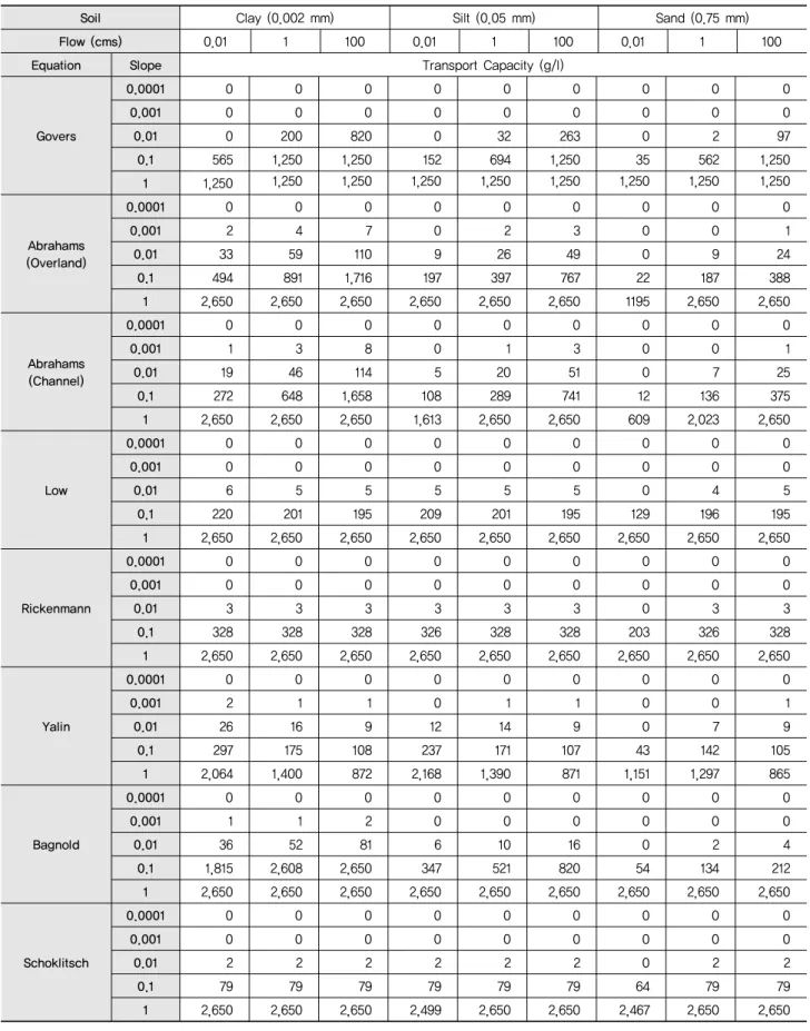
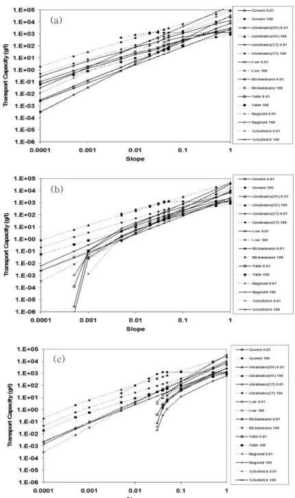
2. Sensitivity to Slope, Flow, and Particle Size The sensitivity analysis showed that sediment transport capacity estimates were more sensitive to slopes than flow discharges and sediment particle sizes (Table 3 and Fig. 2).
The theoretical maximum sediment concentration of 2,650 g/l was applied for all transport capacity estimates made using the equations, whereas 1,250 g/l was applied in the case of the Gover equation based on the observation made by Govers (1992) (Table 3). In Fig. 2, however, the responses of the transport capacity estimations to changes in slopes, flow discharges, and particle sizes were depicted without the consideration of the theoretical maximum sediment concent- ration so as to more extensively exhibit the behavioral of the equations. Overall, the Rickenmann, Bagnold, and Abrahams equations produced relatively great sediment transport capacity estimates, while the Govers and Yalin equations gave relatively small transport capacity estimates across different slopes, flow discharges, and particle sizes (Table 3). The Yang equation provided unrealistic (negative) sedi-
ment concentration estimates for small particles such as clay and silt due to its use of logarithms, thus its sediment transport capacity estimates are not included in this analysis.
In the case of the Schoklitsch equation, the sediment transport capacity was largely controlled by slope, and the impact of flow discharge and particle size on the transport capacity estimates were minimal. All the equations showed similar sensitivity to slope (Fig. 2). However, the different intercepts in the figures indicate that they will provide different sediment transport capacity estimates for the same soil.
The equations provided zero or negligible sediment transport capacity estimates when slopes were equal to or less than 0.001 (0.1 %), and they gave the theoretical maximum concentration (2,650 g/l) when slopes were equal to or greater than 1 (100 %), except for the Yalin and Abrahams equations, indicating applicable slope ranges of the equations are between 0.001 and 1. Sediment concent- rations calculated using the Low, Rickenmann, and Schoklisch equations were relatively insensitive to flow discharges and particle sizes at all the slopes, whereas Abrahams and Bagnold equations were most sensitive to flow discharge and particle sizes, respectively. The Govers equation gave zero sediment concentration when flow is equal to or less than 0.01 cms and slopes are less than 0.01 (1 %). The transport capacity estimates were made using the Yalin equation were sensitive to all the three factors considered:
slopes, flow discharges, and particle sizes. Overall, the Yalin and Abrahams equations that employ the Shield parameter and shear velocity were expected to be most applicable to various topography, flow, and soil diameters.
It is interesting to find that transport capacity estimated using the Yalin and Low equations decreased with increase in flow discharge for clay and silt due to the complicated relationship of the transport capacity to the characteristic diameter (D50), the hydraulic radius, and the Shield parameter as formulated in the equations. This unexpected results reflects the fact that the equations were originally proposed for sand, thus its application to pure clay and silty soils should be carefully implemented. As expected, all the equations provided the greater transport capacity for fine particles (clay) than coarse ones (sand). The transport capacity estimated using the Govers and Abrahams equations was most sensitive to changes in flow discharge.
Table 3 Sensitivity of the sediment transport capacity estimates to slopes, flow discharges, and particle sizes
Soil Clay (0.002 mm) Silt (0.05 mm) Sand (0.75 mm)
Flow (cms) 0.01 1 100 0.01 1 100 0.01 1 100
Equation Slope Transport Capacity (g/l)
Govers
0.0001 0 0 0 0 0 0 0 0 0
0.001 0 0 0 0 0 0 0 0 0
0.01 0 200 820 0 32 263 0 2 97
0.1 565 1,250 1,250 152 694 1,250 35 562 1,250
1 1,250 1,250 1,250 1,250 1,250 1,250 1,250 1,250 1,250
Abrahams (Overland)
0.0001 0 0 0 0 0 0 0 0 0
0.001 2 4 7 0 2 3 0 0 1
0.01 33 59 110 9 26 49 0 9 24
0.1 494 891 1,716 197 397 767 22 187 388
1 2,650 2,650 2,650 2,650 2,650 2,650 1195 2,650 2,650
Abrahams (Channel)
0.0001 0 0 0 0 0 0 0 0 0
0.001 1 3 8 0 1 3 0 0 1
0.01 19 46 114 5 20 51 0 7 25
0.1 272 648 1,658 108 289 741 12 136 375
1 2,650 2,650 2,650 1,613 2,650 2,650 609 2,023 2,650
Low
0.0001 0 0 0 0 0 0 0 0 0
0.001 0 0 0 0 0 0 0 0 0
0.01 6 5 5 5 5 5 0 4 5
0.1 220 201 195 209 201 195 129 196 195
1 2,650 2,650 2,650 2,650 2,650 2,650 2,650 2,650 2,650
Rickenmann
0.0001 0 0 0 0 0 0 0 0 0
0.001 0 0 0 0 0 0 0 0 0
0.01 3 3 3 3 3 3 0 3 3
0.1 328 328 328 326 328 328 203 326 328
1 2,650 2,650 2,650 2,650 2,650 2,650 2,650 2,650 2,650
Yalin
0.0001 0 0 0 0 0 0 0 0 0
0.001 2 1 1 0 1 1 0 0 1
0.01 26 16 9 12 14 9 0 7 9
0.1 297 175 108 237 171 107 43 142 105
1 2,064 1,400 872 2,168 1,390 871 1,151 1,297 865
Bagnold
0.0001 0 0 0 0 0 0 0 0 0
0.001 1 1 2 0 0 0 0 0 0
0.01 36 52 81 6 10 16 0 2 4
0.1 1,815 2,608 2,650 347 521 820 54 134 212
1 2,650 2,650 2,650 2,650 2,650 2,650 2,650 2,650 2,650
Schoklitsch
0.0001 0 0 0 0 0 0 0 0 0
0.001 0 0 0 0 0 0 0 0 0
0.01 2 2 2 2 2 2 0 2 2
0.1 79 79 79 79 79 79 64 79 79
1 2,650 2,650 2,650 2,499 2,650 2,650 2,467 2,650 2,650
Fig. 2 Sensitivity of sediment transport capacity estimates to slopes: (a) clay, (b) silt, and (c) sand (the numbers added to the equation names represent flow (cms) in the legend)
3. Sensitivity to Soil Texture
The empirical equation that Skaggs et al. (2001) proposed was utilized in estimating the cumulative particle size distribution of sediment particles based on soil texture. The shear Reynolds number that controls a critical Shield parameter is a function of the characteristic diameter (i.e.
D50 or R50=D50/2) of sediment particle. The sensitivity of the characteristic radius (or diameter) to soil texture was investigated and represented in Table 4 and Fig. 2. The analysis showed that sandy loam had the widest characteristic radius range, but silt had the narrowest one. In the case of R50, sand and silt had the largest and smallest sediment particle radius, respectively (Table 4). In addition, the
(a)
(b)
(c)
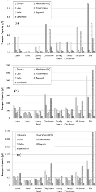
Fig. 4 Sediment transport capacity calculated using characteristic diameters estimated using the method of Skaggs et al.
(2001). (flow of 0.1 cms: (a) slope of 0.001 (0.1 %), (b) slope of 0.010 (1 %), (C) slope of 0.100 (10 %))
Table 4 Characteristic sediment particle sizes for different soil texture in the empirical equation proposed by Skaggs et al. (2001) Characteristic
Radius Loam Sand Loamy Sand Clay Loam Sandy Loam Sandy Clay
Loam Silt Loam Silt
R30 2 70 34 1 10 12 2 1
R40 9 86 41 1 20 22 4 1
R50 19 101 48 6 32 30 8 1
R90 127 187 87 44 182 67 43 13
Unit: µm; Rxx: radius of sediment particles that by mass passes a sieve mesh with an opening equal to xx µm
Fig. 3 Cumulative sediment particle size distributions for different soil textures in the empirical equation proposed by Skaggs et al. (2001)
cumulative mass fraction distributions of sediment particle were distributed between those of sand and silt in an S shaped curve except for that of silt (Fig. 3).
The characteristic diameters were determined for each soil texture using Equations 7 to 13, and then incorporated into the transport capacity equations to investigate sensitivity of capacity estimates to soil texture (Fig. 4). For simplicity of the analysis, flow discharge was fixed to 0.10 cms while slope varied from 0.001 (0.1 %) to 0.1 (10 %). All the equations provided the greatest transport capacity for silt and the least capacity for sand regardless of slopes. The soil textures can be arranged in order of increasing sediment transport capacity estimated using the equations: silt (0.52)
> clay loam (0.25) > silt loam (0.42) > loam (0.34) > sandy clay loam (0.25) > sandy loam (0.24) > loamy sand (0.10) >
sand (0.03). The numbers in the parentheses represent K factor (soil erodibility) of Universal Soil Loss Equation (USLE) proposed by Stewart et al. (1975). The comparison of the equation’s estimates and the K factor values for the soil textures showed good overall agreement between transport capacity and soil erodibility, except for clay loam, implying
the soundness of the methods employed to estimate sediment transport capacity based on soil texture in this study.
When slopes were set to 0.01 (1 %) and 0.10 (10 %), the Bagnold equation provided the greatest difference between the transport capacity estimates made for sand (minimum) and clay loam (or silt, maximum), but the Scholitsch gave the least difference. In other words, the Bagnold equation was most sensitive to soil texture, followed by the Govers, Abrahams, Rickenmann, Yalin, Low, and Scholitsch equa- tions. When slope was set to 0.001 (0.1 %), on the other hand, the Abrahams was most responsive to soil texture, followed by Yalin and Bagnold, and transport capacity calculated using the other equations were negligible (less than 0.1 g/l).
Overall, the Bagnold, Abrahams, Yalin, and Govers equations were more sensitive to soil texture than were the others.
Ⅳ. SUMMARY AND CONCLUSIONS
This study investigated sensitivity of sediment transport capacity calculated using eight equations to slopes, flow discharges, particle sizes, and soil textures. The sensitivity analysis demonstrated that the sediment transport capacity estimates were much more responsive to slope than discharge, particle sizes, and soil texture. All the equations provided zero sediment concentration when slope was shallower than 0.001 (0.1 %), while they gave sediment concentration greater than the theoretical maximum of 2,650 g/l in the case of slope greater than 1.00 (100 %), except for the Yalin and Abrahmas equations, indicating that their applicable slopes were between 0.001 (0.1 %) and 1.00 (100 %). The Abrahams equation (2001) was most responsive to flow discharge, and the Bagnold equations (1980) were most sensitive to particle sizes and soil textures. The Low, Rickenmann (1990), and Schoklitsch equations (1962) were relatively insensitive to flow rates, indicating their poor applicability. The Yang equation (1973) often provided negative values due to the logarithm used in the equation. The Yalin (1963) and Low equations (1989) showed unexpected sensitivity to flow discharge when applied to silt and clay. Overall, the Abrahmas equation showed the widest applicability in estimating sediment transport capacity. These sensitivity analysis results would be useful in selecting transport capacity equations appropriate to a watershed landscape of interest.
REFERENCES
1. Abrahams, A., G. Li, C. Krishnan, and J. F. Atkinson, 2001. A sediment transport equation for interrill overland flow on rough surfaces. Earth Surface Processes and Landforms 26:
1443-1459.
2. Alonso, C. V., W. H. Neibling, and G. R. Foster, 1981. Esti- mating sediment transport capacity in watershed modelling.
Transaction of ASABE 24: 1211-1220.
3. ASCE, 2006. Sedimentation Engineering. ASCE Manuals and Reports on Engineering Practice No. 54. Reston, V.A.: ASCE.
4. Bagnold, R. A. 1966. An approach to the sediment transport problem from general physics. The Physics of Sediment Transport by Wind and Water: A Collection of Hallmark Papers by RA Bagnold, 231-291.
5. Bagnold, R. A., 1980. An empirical correlation of bedload transport rates in flume and natural rivers. Proceedings of the Royal Society of London. Series A, Mathematical and Physical Sciences 372(1751): 453-473.
6. Beasley, D. B., and L. F. Huggins, 1981. ANSWERS user's manual. Report No. EPA-905/9-82-001.
7. DiToro, D. M., 2001. Sediment Flux Modeling. New York, N.Y.: John Wiley & Sons.
8. Dunne, T., and L. B. Leopold, 2002. Water in Environmental Planning. 2nd ed. San Francisco, C.A.: W. H. Freeman Company.
9. EPA, 2003. Developing water quality criteria for suspended and bedded sediments (SABS), Potential Approaches. Washington D.C.: EPA.
10. EPA, 2007. National Water Quality Inventory: Report to Congress, 2002 Reporting Cycle. Washington D.C.: EPA.
11. Fooladmand, H. R., and A. R. Sepaskhah, 2006. Improved estimation of the soil particle-size distribution from textural data. Biosystems Engineering 94(1): 133-138.
12. Foster, G. R., D. C. Flanagan, M. A. Nearing, L. J. Lane, L. M.
Risse, and S. C. Finkner, 1995. Hillslope erosion component.
In USDA-Water Erosion Prediction Project (WEPP), Technical Documentation. West Lafayette, IN.: USDA-ARS-MWA.
13. Foster, G. R., and L. D. Meyer, 1972. A closed-form erosion equation for upland areas. In H. W. Shen (ed) Sedimentation:
Symposium to honor Prof. H. A. Einstein. Colorado State University, Ft. Collins. C.O.: 12.1-12.19.
14. Frinkner, S. C., M. A. Nearing, G. R. Foster, and J. E. Gilley, 1989. A simplified equation for modeling sediment transport capacity. Transactions of ASABE 32(5): 1545-1550.
15. Govers, G., 1990. Empirical relationships for the transport capacity of overland flow. Erosion, Transport and Deposition Processes. Jerusalem, IAHS Publication 189: 45-63.
16. Govers, G., 1992. Evaluation of transporting capacity formulae
for overland flow. Chapter 11. In: Parsons, A.J., Abrahams, A.D. (Eds.), Overland Flow Hydraulics and Erosion Mechanics.
UCL Press, London, pp. 243-273.
17. Guy, B. T., W. T. Dickinson, and R. P. Rudra, 1992. Evaluation of fluvial sediment transport equations for overland flow.
Transactions of ASABE 35(2): 545-555.
18. Haan, C. T., B. J. Barfield, and J. C. Hayes, 1994. Design hydrology and sedimentology for small catchments. Elsevier.
19. Her, Y. G., M. S. Kang, and S. W. Park, 2006. Estimating USLE soil erosion through GIS-based decision support system. Journal of the Korean Society of Agricultural Engineers 48(7): 29-40.
20. Her, Y., 2011. HYSTAR: Hydrology and Sediment Transport Simulation using Time-Area Method. PhD Dissertation, Virginia Polytechnic Institute and State University.
21. Hessel, R., and V. Jetten, 2007. Suitability of transport equations in modelling soil erosion for a small Loess Plateau catchment. Engineering Geology 91: 56-71.
22. Jetten, V., 2002. LISEM (Limburg Soil Erosion Model) User Manual, ver. 2.x. Utrecht Center for Environment and Landscape Dynamics, Netherlands.: Utrecht University.
23. Julien, P. Y., 1995. Erosion and Sedimentation. Cambridge, UK: Cambridge University Press.
24. Kang, M., S. Park, S. Im, and H, Kim, 2003. Computing the half-month rainfall-runoff erosivity factor for RUSLE. Journal of the Korean Society of Agricultural Engineers 45(3): 29-40.
25. Lee, E. J., Y. K. Cho, S. W. Park, and H. K. Kim, 2006.
Estimating soil losses from Saemangeum watershed based on cropping systems. Journal of the Korean Society of Agricultural Engineers 48(6): 29-40.
26. Low, H. S., 1989. Effect of sediment density on bed-load transport. Journal of Hydraulic Engineering 115: 124-138.
27. Meyer, L. D. and W. H. Wschmeier, 1969. Mathematical simulation of the process of soil erosion by water. Transactions of the ASABE 12, 572-580.
28. Misra, R. K., and C. W. Rose, 1996. Application and sensitivity analysis of process-based erosion model GUEST. European Journal of Soil Science 47(4), 593-604.
29. Morgan, R. P. C., J. N. Quinton, R. E. Smith, J. W. Poesen, K.
Auerswald, G. Chisci, D. Torri, and M. E. Styczen, 1998a. The European soil erosion model (EUROSEM): A dynamic approach for predicting sediment transport form fields and small catchments. Earth Surf. Process. Landforms 23: 527-544.
30. Morris, G. L., and J. Fan, 1998. Reservoir Sedimentation Handbook. New York, N.Y.: McGraw-Hill.
31. Nearing, M. A., G. R. Foster, L. J. Lane, and S. C. Finker, 1989.
A process-based soil erosion model for USDA-Water Erosion Prediction Project technology. Transactions of the ASABE 32(5): 1587-1593.
32. Rickenmann, D., 1991. Hyperconcentrated flow and sediment transport at steep slopes. Journal of Hydraulic Engineering 117(11): 1419-1439.
33. Schoklitsch, A., 1962. Handbuch des Wasserbaues (Third Edition). Springer-Verlag, Vienna, Austria.
34. Skaggs, T. H., L. M. Arya, P. J. Shouse, and B. P. Mohanty, 2001. Estimating particle-size distribution from limited soil texture data. Soil Science Society of American Journal 65(4):
1038-1044.
35. Silburn, D. M., and R. J. Loch, 1989. Evaluation of the CREAMS model. I. Sensitivity analysis of the soil erosion/
sedimentation component for aggregated clay soils. Australian Journal of Soil Research 27: 545-561.
36. Song, C. S., and S. Y. Lim, 2014. Prediction of sediment according to type of rural canal. Journal of the Korean Society of Agricultural Engineers 56(6): 121-128.
37. Stewart, B. A., D. A. Woolhiser, W. H. Wischmeier, J. H. Caro, and M. H. Freere, 1975. Control of water pollution from cropland. Vol. 1, Report EPA-600. US Environmental Protection Agency, Washington DC, USA.
38. USDA, 1987. Soil Mechanics Level 1: Module 3 – USDA Textural Soil Classification – Study Guide (revised February 1987). Soil Conservation Service, United States Department of Agriculture.
39. US Department of the Interior, 2006. Erosion and Sedi- mentation Manual. Denver, C.O.: U.S. Department of the Interior, Bureau of Reclamation, Technical Service Center.
40. Wilber, D. H., and D. G. Clarke, 2001. Biological effects of suspended sediments: A review of suspended sediment impacts on fish and shellfish with relation to dredging activities in estuaries. North American Journal of Fisheries Management 21: 855-875.
41. Woolhiser, D. A., R. E. Smith, and D. C. Goodrich, 1990.
KINEROS, A kinematic runoff and erosion model: Documen- tation and user manual. U.S. Department of Agriculture:
Agricultural Research Service.
42. Yalin, M. S., 1963. An expression for bed-load transportation.
Journal of Hydraulic Division, Proceeding of the American Society of Civil Engineers 89(3): 221-250.
43. Yang, C. T., 1973. Incipient motion and sediment transport.
Journal of the Hydraulics Division 99(10): 1679-1704.
44. Yang, C. T. and J. B. Stall, 1974. Unit stream power for sediment transport in alluvial rivers. REs. Rep. 88, Water Resources Center, University of Illinois, Urbana, Illinois, pp. 38.
45. Young, R. A., C. A. Onstad, D. D. Bosch, and W. P. Anderson, 1989. AGNPS: A nonpoint-source pollution model for evaluating agricultural watersheds. Journal of Soil and Water Conservation 46(2): 168-173.