An Object-Oriented Programming for the Boundary Element Method in Plane Elastostatic Contact Analysis
김 문 겸† 윤 익 중*
Kim, Moon Kyum Yun, IkJung
···
요 지
본 논문에서는 경계요소법으로 평면 탄성 접촉문제를 해석하기 위하여 객체지향기법을 이용하여 프로그램을 구성하였 다. 개발된 프로그램의 상세는 UML을 통하여 기술함으로써, C++로 구현된 프로그램이 일반적인 객체지향기법을 통해 구 현될수 있도록 하였다. 개발된 프로그램은 접촉해석의 비선형성과 모퉁이 문제를 포괄할 수 있도록 추상화된 객체로 구현 되었다. 접촉해석에 관련된 객체의 상세를 기술하였으며, 수치해석 예제를 통하여 개발된 프로그램의 정확성을 검증하였다.
핵심용어 : 객체지향 프로그래밍, 경계요소법, 접촉해석, UML, C++, 평면 정적 탄성
Abstract
An object oriented programming(OOP) framework is presented to solve plane elastostatic contact problems by means of the boundary element method(BEM). Unified modeling language(UML) is chosen to describe the structure of the program without loss of generality, even though all implemented codes are written with C++. The implementation is based on computational abstractions of both mathematical and physical concepts associated with contact mechanics involving geometrical nonlinearities and the corner node problems for multi-valued traction. The overall class organization for contact analysis is discussed in detail. Numerical examples are also presented to verify the accuracy of the developed BEM program.
Keywords : object-oriented programming, boundary element method, contact analysis, unified modeling language, C++
···
†책임저자, 종신회원․연세대학교 사회환경시스템공학부 교수 Tel: 02-2123-7504 ; Fax: 02-364-5300
E-mail: [email protected]
* 연세대학교 사회환경시스템공학부 박사과정
∙이 논문에 대한 토론을 2011년 6월 30일까지 본 학회에 보내주시 면 2011년 8월호에 그 결과를 게재하겠습니다.
1. Introduction
The stress developed on the contact surface between multi-bodies have been of great concern in the design of mechanical systems. Analytical solutions for these contact problem are the product of highly sophisticated mathematical analyses for idealized model configura- tions, and in many real situations it is impossible to find a suitable model for an exact solution according to Karami(1989) and Johnson(1985).
On the basis of limited analytical approaches and the advent of high-speed computers, a great deal of
work has been done on the use of numerical methods, such as the finite element method(FEM) and the boundary element method(BEM). The contact problem is essentially a boundary phenomenon that affects the distribution of stress and displacements in the vicinity of the boundary of the contacting bodies (Hertz, 1896). In this sense, the BEM offers an intrinsic advantage in treating contact problems. The BEM was first applied to the contact problem by Andersson et al.(1980), who used constant elements in two-dimensional frictionless problems. Other papers on the BEM for 2D contact problems are available
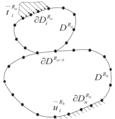
Fig. 1 Configuration of the contact problem (Karami, 1993; Olukoko et al., 1993; Paris et al.,
1995; Huesmann et al., 1995; Lorenzana et al., 1998; Aliabadi, 2002).
Most computer programs for BEM(Brebbia et al., 1992; Becker, 1992; Gallego et al., 1993; 1994;
Beer, 2001; Paris et al., 1997, Gao et al., 2000) have been written with procedure-oriented- programming (POP). These programs work quickly and give good results at the expense of conveniences in maintenance and the possibility of expanding the codes. Additionally, POP is not proper programming concept for mani- pulating complex data, which is unavoidable to sovle modern engineering problems. In recent years, the application of object-oriented programming(OOJ) to numerical applications has received increasing attention because its key features (data encapsulation, message passing, hierarchical code organization, inheritance and polymorphism) can produce a robust and generic code with enhanced modularity, improved reusability and complex data structures that lead to the fastest prototyping and easiest debugging of new code in the FE field since 1990. In recognition of some of the superiorities of OOP, some research has been conducted to import OOP concepts into BE fields(Noronha et al., 1997; Christian, 1998; Friedrich, 1998; Wang et al., 1999; Marczak, 2004; Marczak, 2006; Qiao, 2006), but there has been no reported work, which directly treats contact problem by BEM. Solving contact problem by BEM requires very sophisticate data algorithms such as contact detection(Kim et al., 2009).
Therefore, the remainder of this paper consists of developing an BE program with OOP and verifying it.
For the sake of generality and clarity, the unified modeling language(Fowler, 2004) is used to describe conceptual components of the developed BE program, which is written with C++. Several objects are designed to manipulate complex data of contact problem. To show the capability of the developed code treats the corner node problem of the BEM, the proposed architecture will be closely dissected by collaboration diagrams. Conforming contact problem and non-conforming problem will be solved to show
the capability of developed program manipulating complex data structure and finding an accurate solution.
2. BE formulation for contact analysis
2.1 BI formulation of multiple regions
In contact analysis, the boundary element procedure can be applied to each sub region in turn, as if they were independent of one another. The final set of equations for the entire region can be obtained by assembling the set of equations for each sub region using the compatibility of displacements and traction equilibrium between the common interfaces.
For simplicity, consider the interaction between the two bodies, ( ), occupying the domain,
, and having the boundary, , represented in Fig. 1. The external loads were visualized as traction and restraints in the displacements. Then the boundary conditions of the problem are written as:
∈ ∈ (1) where
∪ , ∅
∪ ,
is Dirichlet boundary condition, and
is Neumann boundary condition.
In the absence of body forces, the field equations of each body can be expressed in terms of boundary integrals by means of Somigliana's Identity: a point
in the domain can be written in the form :
(2)
where the displacements and stress vector solution of the Kelvin problem for plane elastostatic probelms,
and , assuming homogeneous and linear elastic behavior, can be written as Eqs (3) and (4).
′ ′
′
′
(3)
′
′
′ (4)
′ and ′ in the plane strain and
′ × and ′ in the plane stress. is the elastic constants and is the poisson's ratio of the body , and is the distance between the points and , is the outward normal at point on the . is usually called the free term of the equation that varies depending on the smoothness of the boundary
. The boundary is the area not in contact, and
is the area in contact.
The boundary integral equations of multi-bodies are discretized separately. The resulting sets of matrices can be written as:
(5)
where are matrices whose coefficients represent integrations of
over elements, and are matrices whose coefficients represent the integration of . Vectors and represent boundary values of displacements and traction. In the contact region, the
systems of equations share the boundary variables of the problem. Thus, these equations are coupled and must be solved simultaneously for any given com- bination of boundary conditions. Various assembly methods have been proposed, but here we follow the substructure techniques of Gao et al.(2000). After applying the boundary conditions, the resulting system equations can be written in Eq. (6).
(6)
where are the remaining boundary unknowns, are known values obtained from the product of the specified boundary conditions and the corresponding matrix coefficients, and is a matrix of known coefficients.
2.2 Boundary and contact conditions
The mutually exclusive boundary condition is specified for BE problems to solve integral equations.
If a closed domain that consists of number of nodes lies in plane, the final system matrix has 22
× 2× equations in the system, with of them placed at the Dirichlet boundary and at the Neumann boundary . However, the number of unknowns is unknown a priori because boundary conditions of the nodes on the contact interface
∩ depend on the applied load. For the first iteration to solve the non-linearity based on the boundary condition that changes under a load, it is assumed that all node pairs in contact are stuck together. Thus, the unknown variables associated with each node on the contact interface will be 4
∩2×
∩2×
∩
. An approach to reducing unknowns is to impose contact constraints on the contact interface by using compatibility equations and equilibrium conditions (7) which is written:
(7)
where the subscripts in Eq. (7), and , mean
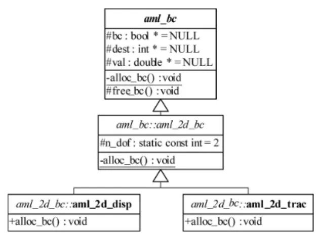
Fig. 2 Hierarachy model of aml_bc class normal direction and tangential direction.
3. OOP for contact analysis with BEM
OOP has become a common paradigm in many software development fields, including scientific and engineering software(Stroustrup, 1997). The diffusion of the use of OOP languages in engineering is due to a number of factors, most of them deeply rooted in the demand for extensibility and reusability of the codes without the demanding costs associated with the development of new software or unwanted changes in codes that are successfully tested and used. The main objective of this section is to construct a concrete framework for the BE contact analysis program with well-structured classes utilizing the key concepts of OOP; encapsulation, inheritance, polymorphism and late bindings(McMonnies et al., 1995; Friedrich, 1998).
3.1 Design data structures
Object design is the fundamental step in OOP. The utilization of OOP in BE contact analysis is mainly focused on constructing data structures of objects and their methods. All implemented codes are written with C++ because FORTRAN does not support an array of pointers(Chapman, 2007), which plays a crucial role in manipulating data information efficiently, and FORTRAN provides only restricted OOP.
3.1.1 Boundary condition classes
Two simple classes, aml_2d_disp and aml_2d_ trac, are derived to manage the information for boundary conditions from the base class aml_2d_bc represented in Fig. 2. These classes impose the boundary condi- tions of the entire domain into a discretized mesh and provide destination arrays to assemble the final system equation (6). The only difference between the aml_2d_disp class and aml_2d_trac class is the initialization method, alloc_bc(…). This method is overloaded so that traction is initialized as a free surface and displacement remains unknown for each
degree of freedom.
3.1.2 Node and element classes
When sharp corners or edges are existed on mesh, then the traction of the extreme nodes on the corner elements is multi-valued, although displacement is uniquely defined at each node, because the outward normal is different on each side of a point. Consider the example of an elastostatic problem in Fig. 3, Dirichlet boundary condition with a prescribed value on the left side are unique, and the Neumann conditions on the extreme node of the upper side and bottom side are multi-valued as shown. The free surface is treated as zero prescribed traction. The traction value of each extreme node that belongs to adjacent elements will be treated as independent variables, and the displacement value is unique. This phenomenon induces conflicts within the iteration loops in the assembly procedure for constructing the final system equation because application of the boundary conditions is performed at the node level, but the assembly loop iterations are conducted at the element level. Furthermore, augmented equations for displacements are provided at the node, but aug- mented equations for traction, which are required to construct the final system equations, are given at the element level.
To manipulate this notorious phenomenon, called corner problem in BEM, setting the unified interface to approach boundary condition object is essential. In order to resolve corner problem, aml_2d_node class is
Fig. 3 A configuration of the discretization of BE region
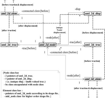
Fig. 4 Association diagram of aml_node and aml_elem class
Fig. 5 Hierarchy model of aml_node class only devised to have a pointer of the instance of the
aml_2d_disp class and two pointers of the instance of
the aml_2d_trac class. This technique, called data hiding, guarantees that the instance of the boundary classes cannot be accessed by other instance but the instance of aml_2d_node object, and provides unique path to get the boundary indicators. All aml_2d_bc instances are referred with the pointers to indicate directly the objects, to increase computational efficiency and to save memory. For an aml_2d_elem class, the only path to get boundary information is the interface of aml_node class is calling the set-get methods of the aml_2d_bc instance. This data encapsulation technique enables a unified path to boundary condition instances. This approach is shown in Fig. 4. Under the same architecture, aml_node class and aml_elem
Fig. 6 Hierarchy model of aml_node class
Fig. 7 Hierarchy model of aml_region class
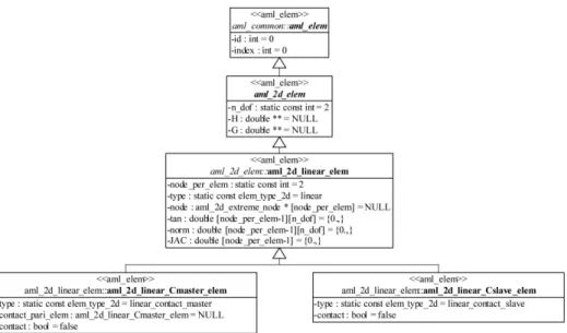
class are also declared, as in Fig. 5 and 6.
The aml_elem class must be able to evaluate integral constants by calling its abstract method virtual void evaluate_integral_const(···). Most complex numerical BE algorithms lie in this method, but to operate this, the incidence array of elements is determined a priori. Therefore, any element class should be derived with a suitable shape function from its base class and have a modified implementation of the virtual void evaluate_ integral_const(···). In this article, aml_2d_linear_elem is derived for a linear element and expanded to aml_ 2d _linear_ Cmaster_
elem and aml_2d_linear_Cslave _lem to treat contact algorithm.
3.1.3 Region classes
Most of contact problem is conducted with the interaction between multi-bodies. Each body is recognized as a sub-region that has its own material properties and mesh with nodes and elements. The hierarchy model of aml_region_class is designed to reflect this, represented in Fig. 7.
3.1.4 Bem classes
Finally, the wrapping class, aml_bem is designed to pass the message in the proper order. This wrapping class merges all complex implementation of each classes. The hierarchy model of the class is shown in Fig. 8.
Fig. 8 Hierarchy model of aml_bem class
Fig. 9 Hierarchy model of aml_bem class 3.2 Put it all together
The main program for plane elastostatic contact analysis starts by creating an instance of the aml_2d_bem class. After creating the instance, the solution procedure is processed as following steps.
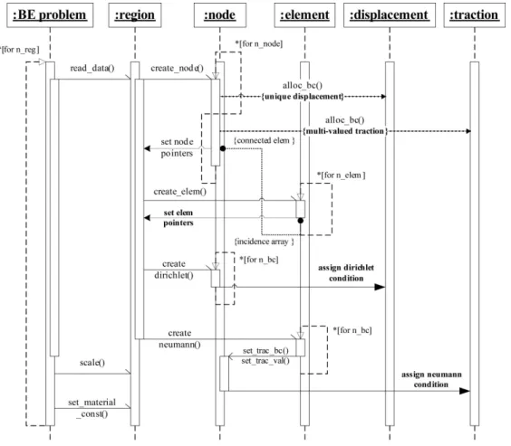
3.2.1 Preprocessing
In this segment, sets of objects are dynamically
established to store nodal coordinates, element con- nectivity, material properties, boundary condition indicators and prescribed boundary condition. Objects are allocated and set in 4 main loops. This procedure is represented in Fig. 9.
•Regional loop : allocates memory for sub regions;
•Nodal loop : allocates memory for node of a sub region and reads boundary coordinates. At this stage, memory for Dirichlet condition is allocated;
Fig. 10 Collaboration diagram of the integral constants evaluation segment
Fig. 11 Collaboration diagram of assembly of system equations
Fig. 12 A conforming contact problem
•Elemental loop : allocates memory for each element of a subregion and reads the incidence array;
•Dirichlet condition loop : assigns Dirichlet condi- tions to nodes;
•Neumann condition loop : assigns Neumann conditions to element nodes;
3.2.2 Evaluation of integral constants
Integral constants are evaluated by the virtual void evaluate_integral_const(…) method, which is declared in a base class method and dynamically bound to its derived class during execution depending on what type of boundary element is used. In each child class, the member function must be modified accordingly. These methods are invoked as shown Fig.10.
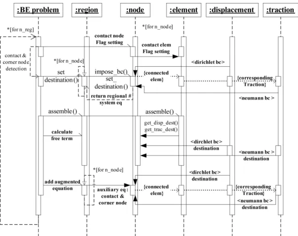
3.2.3 Assemble system equations
Before the generating final system equations, the boundary condition must be set up according to all boundary indicators associated with a node because the final system equation is assembled by gathering element contributions to the collocation node. After setting boundary condition indicators of the node, the assembling procedure is processed as in Fig. 11.
3.2.4 Solve system equations
Finally, the virtual void solve(…) method of aml_
2d_bem class calls a generic function to solve the system equations and checks the contact state. If the contact state is satisfied, the final results are printed. Three contact indicators are listed below:
• no edge overlaps;
• no tensile stress between contact elements;
• friction slips.
4. Numerical examples
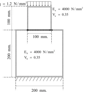
To verify the accuracy of the developed program, non-conforming contact problem and conforming contact problem were solved and the results are given. Fig. 12. shows the discretized geometry, properties
and boundary conditions of the conforming frictionless contact problem.
Analytical solution for contact problems has been limited to simple cases. Moreover, proving the existence and uniqueness of the solution for a contact problem in the general setting has still not been achieved (Wriggers, 2002). These two limitations make it difficult to verify numerical methods, including FEM and BEM, for contact problems. Even though the rigorous verification is almost impossible and how the model for a specific problem behaves as parameters is still not well understood, FEM has been utilized to solve real world problems and has been very successful in most applications. In this context, the FEM solutions can be used for comparison because the proposed BEM algorithms are supposed to be equivalent, if not better, than the FEM with regard to accuracy. The ABAQUS FE program(2007) was employed to perform contact analysis of the proposed example, and the meshes were designed with a similar discretization to that of the BE models. A Lagrangian multiplier formulation was used to represent the contact region of the model. The BE mesh of this model consists of 298 two node linear elements. The distribution of the contact stresses along the contact zone is shown in Fig. 13 and is compared with the one obtained by FEM. The contact stress results are in very good agreement. Similar
Fig. 13 Contact stress along the contact zone
Fig. 14 A non-conforming contact problem
Fig. 15 Contact stress along the contact zone
contact stress behavior can be found in the published result by Paris et al.(1995).
Fig. 14. shows conformal contact problem, classified into the Hertz contact problem. To solve this example, the quarter-cylinder is modeled with 42 discrete linear contact boundary elements. The distribution of the contact stresses along the contact zone is shown in Fig. 15 and is compared with the exact solution. The contact stress results are in very good agreement.
5. Conclusion
In this paper, an object-oriented BEM code was developed to take advantage of the clearly object- oriented nature of boundary elements, especially with respect to property inheritance and function overloa- ding. Furthermore, an array of pointers and the vector template of the C++ language allowed boundary indicators to be accessed directly, including a contact state without any additional programming efforts.
Plane elastostatic contact problems are decomposed into 5 base classes defined under the OOP framework.
Except for the wrapping class, each object represents real BE problems conditions. To the author’ best knowledge, there is no published work dealing with an OOP approach for contact problems with multi- regions considering corner node problems. The validity and accuracy of the developed BE program were verified by comparisons to the FE solution and the published result.
References
Aliabadi, M.H. (2002) The Boundary Element Method Volume 2, Applications in Solids and Structures, WILEY.
Andersson, T., Frederiksson, B., Persson, B.G.A.
(1980) The Boundary Element Method Applied to Two-Dimensional Contact Problems, in: C. A.
Brebbia(Ed.), Proceedings of the 2nd International Seminar on Recent Advances in BEM, Southampton:
CML Publications, pp.247~263.
Bangyong, K., Yijun, L. (2005) Analysis of 3-D Frictional Contact Mechanics Problems by a Boun- dary Element Method, Tsinghua Science and Techno- logy, 10, pp.16~29.
Becker, A.A. (1992) The Boundary Element Method in Engineering, a Complete Course, London: McGraw- Hill.
Beer, G. (2001) Programming the Boundary Element Method, an Introductionfor Engineers, WILEY, Brebbia, C.A., Dominguez, J. (1992) Boundary
Elements, an Introductory Course. 2nd ed, New York: McGraw-Hill.
Chapman, S.J. (2007) FORTRAN 95/2003 for Scien-
tists and Engineers, McGraw-Hill.
Dassault systems simulia corp. (2007), Abaqus 6.7 User’ manual.
Friedrich, J. (1998) Object Oriented Computer Simulations of Physical Systems using Dual Reci- procity Boundary Element Methodology, Turkish Journal of Electrical Engineering & Computer Sciences, 6, pp.11~22.
Gallego, R., Dominguez, J. (1993) A Two Dim- ensional Boundary Element Code for Time-Domain Formulations using Quadratic Elements II: Tran- sient Elastodynamic Problems, Boundary Elem Commun.
Gallego, R., Dominguez, J. (1994) A Two Dim- ensional Boundary Element Code for Time-Domain Formulations using Quadratic Elements I: Poten- tial Problems, Boundary Elem Commun.
Gao, X.W., Davies, T.G. (2000) 3D Multi-Region BEM with Corners and Edges, International Journal of Solids and Structures, 37, pp.1549~1560.
Hertz, H. (1896) Miscellaneous Papers on the Contact of Elastic Solids, Translated by D.E. Jones, Mac Millan: London.
Huesmann, A., Kuhn, G. (1995) Automatic Load Incrementation Technique for Plane Elastoplastic Frictional Contact Problems using Boundary Element Method, Computers & Structures, 56, pp.733~
744.
Johnson, K.L. (1985) Contact Mechanics, Cambridge University Press.
Karami, G. (1989) A Boundary Element Method for Two Dimensional Contact Problems, Springer-Verlag.
Karami, G. (1993) Boundary Element Analysis of Two-Dimensional Elastoplastic Contact Problems, International Journal for Numerical Methods in Engineering, 36, pp.221~235.
Kim, M.K., Yun, I. (2009) An Efficient Contact Detection Algorithm for Contact Problems with the Boundary Element Method, Computational Structural Engineering Institute of Korea, 22(5), pp.439~
444.
Lorenzana, A., Garrido, J.A. (1998) A Boundary Element Approach for Thecontact Problems Involving Large Displacements, Computer & Structures. 68, pp.315~324.
McMonnies, A., McSporran, W.S. (1995) Developing Object-Oriented Data Structures using C++, Mc Graw-Hill.
Olukoko, O.A., Becker, A.A. (1993) A New Boun- dary Element Approach for Contact Problems with Friction, International Journal for Numerical Methods in Engineering, 36, pp.2625~2642.
Paris, F., Blazquez, A., Canas, J. (1995) Contact Problems with Nonconforming Discretization using Boundary Element Method, Computers & Structures, 57, pp.829~839.
Paris, F., Canas, J. (1997) Boundary Element Method, Fundamentals and Applications, Oxford University Press.
Stroustrup, B. (1997) The C++ Programming Language, MA: Addison-Wesley.
Wriggers, P. (2002) Computational Contact Mech- anics, New York: John Wiley & Sons.
논문접수일 2009년 12월 1일 논문심사일
1차 2009년 12월 7일 2차 2011년 2월 18일 게재확정일 2011년 2월 19일