서론 I.
2 Ziegler-Nichos
Cohen-Coon
, , ,
,
PID [1,2].
[3], PID PI-PD [4], I-PD [5,6], PI+D [7],
. (Genetic Algorithm)
PID [8,9,10]
PID [11].
, .
, ,
,
PI
* (Corresponding Author)
: 2011. 3. 14., : 2011. 4. 11., : 2011. 5. 4.
. ( )
. ( )
. ( )
2 .
( ) PI , Fine
Coarse .
Matlab simulink ,
. . II
1 , III II
, IV
, .
속도제어기의 차 함수화 유도
II. 1
1 . (excitation
magnetic field) , (armature)
() () .
()
(1)
, (2)
.
, ,
A Study on Current, Velocity, Position Gain Tuning Technique of Servo Position Controller using Simulation
* (Ki-Woo Park1)
1Daewon Mechatronics
Abstract: When a servo position controller of a robot or a driving units is composed of a PID controller, servomechanism which is modelled is composed of current, velocity and position control loops. After this model is simulated, the technique operating gain of each controller is suggested. The model consists of current, velocity and position controllers from the inside to the outside gradually. Also, to combine velocity and position controllers with 2 order system, simulation is performed after current controllers are composed, which are able for current loop to work ideally. If a current controller is treated with constant, it is possible for velocity and position controller to consist of controller into 2 order system. The technique is verified by applying T-company servo motor which is much more applied to current, velocity and position controller robots.
Keywords: PID controller, servo mechanism current control loop, velocity control loop, position control loop, 2 order system
Copyright© ICROS 2011
Motor
부하 BL JL Wm Ra La
+ -
e
gConstant field
O
O O
O
+
-
e
ai
aN : 1
1. .
Fig. 1. DC motor and load model.
(1)
(2)
( , : , : ,
: )
(torque, T)
() ,
(3) . (1)~(3)
Laplace (4)~(6) ,
2 .
(3)
( ,
)
(4)
(5)
(6) 2
.
.
(7)
B ,
≈
(8)
(8)
L zero (Approximation) ,
(9) .
≈
(9)
(current control loop) (bandwidth) (velocity control loop)
(bandwidth) 20
, ≪ (Approximation) .
(9) ≪ ,
≈
(10)
2 1
(10) .
(current control loop) (bandwidth) (velocity control loop)
(bandwidth) ,
, .
( ) 1
(1st order lowpass filter)
.
.
.
제어기 설계 III.
전류제어기 설계 1.
()
.
(10) .
(10) .
(11) , () ≈ ,
, R L ,
.
, .
(-3dB) ,
+- +- JS+B
1 ω LS+R1 Kt
Kpi
Kpi
+- +-
Kp Kpv
ωi Io o
Ii
Ke At
2. .
Fig. 2. Velocity control block diagram of servo system of DC motor.
() .
(11) 속도제어기 설계
2.
II 1
2
.
1/20 ,
.
1 ()
. , H(S) , (10) .
()
() .
위치제어기 설계 3.
3
PI .
. 3 N
, J Inertia
. Inertia J Inertia
Inertia (12) .
(12)
PI
(type number) 1 , ,
. Kp
Ki . PI
,
.
Coarse Fine
Coarse
() , Fine
() ()
. 제어 영역의 비례제어
3.1 Coarse ()동조
,
(tuning) . 3
Coarse
() , H(S)
(10) 1 ,
() 2
. ()
Coarse .
() .
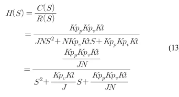
H(S) (13) .
(13)
(13) 2 (14)
() () .
(14)
3.2 Fine 제어 영역의 비례제어() 및 적분제어() 동조
3 Fine
H(S) () ()
(15) .
(15)
(15) Fine ()
,
()≈
()≈
,
()≈
. (15) (16) .
(16)
+- +
- JS+B1 ω Θ
S1 o LS+R1 Kt
Kpi
Kpi +- +- Kp Kpv
ωi Io o
Ii
Ke At
Kp Kpp +- Θi
Θo
N1
3. .
Fig. 3. Position control block diagram of servo system of DC motor.
Fine ()
(17) .
(17)
Coarse
(17) , (17)
() .
3.3. 위치제어기의 Coarse 제어 영역과 Fine 제어 영 역 설정
() ()
, ,
, Fine .
3~ 5
mrad . 4 PI .
Fine
(10mrad ) ()
, ()
( 9, 10, 11)
. Fine
Fine Coarse
. Fine Coarse
.
12, 13 Fine (1mrad)
Coarse ()
.
시뮬레이션 IV.
3 1
. 전류제어기 시뮬레이션 1.
2
5 .
, (backemf) Ke
(zero) , .
(11) () Matlab simulink
,
. 5
, 6, 7
, 8
(-3dB) 10KHz .
(= 6.5),
(BW=10KHz) .
속도 및 위치제어기 시뮬레이션 2.
속도제어이득
2.1 ()동조
(10)
( 1/20) (18), (19)
, , .
Kp +p
SKI
Kpp
위치오차(mrad) ωi
Coarse영역
Fine영역 3~5
4. PI .
Fig. 4. Concept of pi position control.
1. 200 Watt (Tamagawa Seiki) [12].
Table 1. 200 Watt servo motor spec(Tamagawa Seiki).
Motor
Torque Constant (KT) 0.119 N m/A Voltage Constant (KE) 12.4×10⁻³ V/(r/min) Armature Resistance (Ra) 0.4
Armature Inductance (La) 0.6 mH Instantaneous Max. Current (Ip) 31 A
Rated Voltage (Vo) 42 V Rated Current (Io) 6.5 A
Rated Speed (No) 3000 r/min Rated Torque (To) 0.637 N m Rated Output Power 200 W Instantaneous Peak Torque (Tp) 3.64 N m
Max. Speed (N) 4000 r/min Moment of Inertia (JM) 1.64×10⁻⁴ Kg m2 Mechanical time Constant (Tm) 4.7 msec
Electrical Time Constant (Te) 1.5 msec Thermal Resistance (Rth) 1.2 /Watt
Friction Torque (Tf) 4.9×10⁻² N m
Mass 2.2 Kg
Tacho Output Voltage 6 V/Kr/min
0.6X10 S+0.41 6.5
+-
+ Io
Ii
-3
5. .
Fig. 5. Current control loop simulation.
6. . Fig. 6. Current loop simulation step command.
7. .
Fig. 7. Current loop simulation sinusoidal command.
-40 -30 -20 -10 0
Mag nitu de (d B)
102 103 104 105 106
-90 -45 0
Pha se (d eg)
Bode Diagram
Frequency (rad/sec)
8. .
Fig. 8. Bode plot of current loop and bandwidth.
×
(18)
(19) 위치제어 비례이득
2.2 ()동조
(13) (19) ()
() .
× , ×
위치제어 적분이득
2.3 ()동조
(17) 4.2.2 (), ≈
,
() .
× ,( : 380) 2.4 위치제어기의 Coarse 제어 영역과 Fine 제어 영
역 설정
() , ,
, 4 5 mrad Fine .
위치제어기의 시뮬레이션 2.5
(Typical)
9, 10, 11 . 3
, (step), (ramp), (sinusoidal) . ‘1. Proposed PI’
, ‘2. Typical PI’
(typical) PI .
(), ()
, ()
380
12.5( 1/10) .
(10rad)
, (zero)
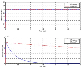
. (0.5rad/sec)
(proposed) 1 0.5 mrad
(typical) PI 3 3 mrad
.
(typical) PI ()
. (0.7rad, sin1t)
2 mrad. , PI 6 mrad.
.
PI (3~4 ) .
11 Fine
5 mrad ( )
() .
0 0.01 0.02 0.03 0.04 0.05 0.06 0.07 0.08 0.09 0.1
-40 -20 0 20 40
Time (sec)
Cur rent (A)
1.Proposed PI 2.Typical PI
0 0.01 0.02 0.03 0.04 0.05 0.06 0.07 0.08 0.09 0.1
-100 0 100 200 300 400
Time (sec)
Vel ocity (rad/
sec)
1.Proposed PI 2.Typical PI
9. , : (10rad), :
, ( ).
Fig. 9. Position Control Loop Simulation, Input: Step Command (10rad), Output: Current, Velocity.
0 0.5 1 1.5 2 2.5 3
0 0.1 0.2 0.3 0.4 0.5 0.6 0.7
Time (sec)
Vel ocity (rad/
sec)
1.Proposed PI 2.Typical PI
0 0.5 1 1.5 2 2.5 3
0 1 2 3 4 5 x 10⁻³
Time (sec)
Pos ition Erro r(rad )
1.Proposed PI 2.Typical PI
10. , : (0.5rad/sec)
, : , .
Fig. 10. Position Control Loop Simulation, Input: ramp(0.5rad/
sec) Command, Output: Velocity, Position Error.
0 1 2 3 4 5 6 7 8 9 10
-1 -0.5 0 0.5 1
Tim e (sec)
Vel ocity (rad/
sec) 1.Proposed PI
2.Typical PI
0 1 2 3 4 5 6 7 8 9 10
-0.01 -0.005 0 0.005 0.01
Tim e (sec)
Pos ition Erro r(rad
) 1.Proposed PI
2.Typical PI
11. , : , 40°sin1t,
1Hz, : , .
Fig. 11. Position Control Loop Simulation, Input: Sinusoidal 40°, sin1t, 1Hz, Output: Velocity, Position Error.
0 0.5 1 1.5 2 2.5 3
0 0.1 0.2 0.3 0.4 0.5 0.6 0.7
Time (sec) Vel
ocity (rad/
sec)
1.Proposed PI 2.Typical PI
0 0.5 1 1.5 2 2.5 3
0 1 2 3 4 5 x 10⁻³
Time (sec) Pos
ition Erro r(rad )
1.Proposed PI 2.Typical PI
12. , : (0.5rad/sec)
, : , .
Fig. 12. Position Control Loop Simulation, Input: ramp(0.5rad/ec) Command, Output: Velocity, Position Error.
0 1 2 3 4 5 6 7 8 9 10
-1 -0.5 0 0.5 1
Time (sec)
Vel ocity (rad/
sec) 1.Proposed PI
2.Typical PI
0 1 2 3 4 5 6 7 8 9 10
-0.01 -0.005 0 0.005 0.01
Time (sec)
Pos ition Erro r(rad
) 1.Proposed PI
2.Typical PI
13. , : , 40°sin1t,
1Hz, : , .
Fig. 13. Position Control Loop Simulation, Input: Sinusoidal 40°, sin1t, 1Hz, Output: Velocity, Position Error.
결론 V.
,
,
, 1 ,
․
. Coarse Fine
Fine
. Fine
() . Coarse
2
.
Matlab simulink ,
(Step Position Command),
(Ramp Command), (sinusoidal
Command) .
참고문헌
[1] J. G. Ziegler and N. B. Nichols, “Optimum setting for automatic controllers,” Trans. ASME, vol. 64, pp. 759- 768, Nov. 1942.
[2] G. H. Cohen and G. A. Coon, “Theoretical consideration of retarded control,” Trans. ASME, vol. 75, pp. 827-834, Jul. 1953.
[3] S. T. Lee and H. S. Cho, “A fuzzy controller for an aeroload simulator using phase plane method,” IEEE Trans. Control System Technology, vol. 9, no. 6 pp. 791- 801, Nov. 2001.
[4] N. Tan, “Computation of stabilizing PI-PD controllers,”
International Journal of Control, Automation, and Systems, pp. 175-184, Jul. 2009.
[5] H. G. Ha, “The design of a pre-compensator for the model-following control in the I-PD control system,”
Journal of KIEE, vol. 18, no. 6, pp. 84-90, Nov. 2004.
[6] S. D. Kim, “Design of the PD controller in the I-PD control system for position control,” Journal of the
Institute of Signal Processing and Systems, vol. 10, no.
4, pp. 262-266, Oct. 2009.
[7] C. S. Jang, J. W. Choi, Y. S. Oh, and S. Chae, “A study on the self-tuning of the design variables and gains using fuzzy PI+D controller,” Journal of Korean Institute of Intelligent Systems, vol. 17, no. 3, pp. 355-367, Jun.
2007.
[8] J. S. Kim, J. H. Kim, J. M. Park, S. M. Park, W. Y.
Choe, and H. Heo, “Auto tuning pid controller based on improved genetic algorithm for reverse osmosis plant,”
Proc. of World Academy of Science, Engineering and Technology, Issue 47, pp. 384-389, Nov. 2008.
[9] D. E. Kim and G. G. Jin, “Tuning rules of the PID controller based on genetic algorithms,” Proc. of the KIEE Summer Annual Conference, pp. 2167-2170, Jul.
2002.
[10] Z. X. Wang, J. J. Yang, S. B. Rho, and T. C. Ahn, “A new design of fuzzy controller for HVDC system with the aid of GAs,” Journal of Control, Automation, and Systems Engineering, vol. 12 no. 3 pp. 175-184, Mar.
2006.
[11] V. Aggarwal, M. Mao, and U.-M. O'Reilly, “A self-tuning analog proportional-integral-derivative (pid) controller,” Proc. First NASA/ESA Conference on Adaptive Hardware and Systems AHS 2006, pp. 12-19, Jun. 2006.
[12] TAMAGAWA SEILI CO. “TRE series DC Servo Motor,”
200Watt. pp. 9-10.
박 기 우
1989 . 2005
. 2006 ~
. 1989 ~2000 .
2001 ~ .
, .