Vol. 19, No. 3 pp. 40-45, 2018
On-line Process Data-driven Diagnostics Using Statistical Techniques
Hyun-Woo Cho
Department of Industrial and Management Engineering, Daegu University
실시간 공정 데이터와 통계적 방법에 기반한 이상진단
조현우
대구대학교 산업경영공학과
Abstract Intelligent monitoring and diagnosis of production processes based on multivariate statistical methods has been one of important tasks for safety and quality issues. This is due to the fact that faults and unexpected events may have serious impacts on the operation of processes. This study proposes a diagnostic scheme based on effective representation of process measurement data and is evaluated using simulation process data. The effects of utilizing a preprocessing step and nonlinear statistical methods are also tested using fifteen faults of the simulation process.
Results show that the proposed scheme produced more reliable results and outperformed other tested schemes with none of the filtering step and nonlinear methods. The proposed scheme is expected to be robust to process noises and easy to develop due to the lack of required rigorous mathematical process models or expert knowledge.
요 약 생산 공정의 다변량 데이터에 기반한 지능적 공정 감시 및 진단 시스템은 조업의 안정성과 고품질의 제품을 달성하고 경쟁력을 유지하기 위해서는 필수적인 업무 중 하나로 간주되고 있는데, 이와 같은 추세는 공정 이상이 발생하는 경우 안정 적이고 경제적인 조업에 큰 영향을 미치는 것에 기인한다. 본 연구에서는 다변량 공정 데이터에 기반한 진단기법을 제시하고 이를 시뮬레이션 공정 데이터를 활용하여 그 성능을 평가하고자 한다. 또한 원 데이터의 전처리 과정의 유무와 비선형 방법 론의 활용이 진단 성능에 마치는 영향을 시뮬레이션 공정에서 제시된 15개의 공정 이상에 대해 평가하였다. 그 결과 제안된 방법론이 신뢰할 만한 결과를 주었으며 다른 비교 방법론인 전처리 과정이 없거나 선형 방법론을 사용한 타 방법론 대비 우월한 성능을 보여주었다. 제시된 방법론은 공정 데이터에 기반한 방법론으로서 공정에 대한 수학적 모델이나 지식 모델에 비하여 상대적으로 모델링이 간편하며 공정 데이터의 잡음에 강건하다는 장점을 가진다.
Keywords : Diagnosis, fault, filtering, multivariate statistical methods, process data
This work was supported by the Daegu University Research Grant, 2013.
*Corresponding Author : Hyun-Woo Cho (Daegu Univ.) Tel: +82-2-850-6540 email: hwcho@daegu.ac.kr
Received December 7, 2017 Revised (1st December 28, 2017, 2nd January 8, 2018) Accepted March 9, 2018 Published March 31, 2018
1. Introduction
Continuous monitoring of industrial processes is quite necessary in order to guarantee process safety and quality issues. Process faults or abnormal events should be detected and diagnosed as soon as possible.
Based on the monitoring results provided appropriate remedial actions are determined and executed in an
on-line basis[1]. The diagnosis is to identify assignable causes of the detected faults. Recently, massive process measurement data can be easily obtained from most of production processes. It has facilitated the use of multivariate statistical approaches to fault diagnosis problems[2]. Multivariate statistical techniques have been utilized in practical issues including principal component analysis (PCA), partial least squares (PLS),
and Fisher discriminant analysis (FDA) [3]-[5].
Nonlinear monitoring techniques have been also developed as extended versions of linear methods.
They have the common things that input data are mapped into nonlinear spaces and then these mapped data are analysed. The use of such a kernel trick enables us to develop various kernel methods such as kernel PCA, kernel PLS and kernel FDA[6]. The selection of linear or nonlinear techniques depends on the problems of interest. In linear case, in general, data can be modeled effectively by both linear and nonlinear techniques. The use of a linear technique in nonlinear case, however, may not represent most of data correctly.
As data measurement and sensing technologies advance, automated on-line data collection has become popular. The availability of such massive data sets has motivated the use of multivariate statistical approaches to diagnosis problems. Diagnosis problems can be treated as classification problems when there are lots of historical data obtained from various faulty conditions.
The multivariate statistical techniques for fault diagnosis, in general, are considered to be easy to implement, computationally efficient, and relatively robust to noise[7]. When data analysis is performed, redundant portions of data may cause masking problem of underlying patterns. Thus preprocessing or filtering of raw data is necessary in order to improve the performance of data analysis. Combined with nonlinear and triangular methods efficient preprocessing step can be added to improve diagnosis results by removing unwanted parts of raw measurement data.
This work proposes an multivariate statistical diagnostic scheme based on nonlinear representation of raw measurement data. To capture fault patterns in reduced spaces a triangular representation of process data is combined with nonlinear methods. This diagnostic scheme is suitable for distinguishing different groups of faults. In this work, a preprocessing or filtering step is added to eliminate unwanted parts of the data. The adoption of a filtering task is expected to
improve the performance of the diagnostic scheme. The performance of the proposed diagnostic scheme is tested and demonstrated using measurement data of a simulation process.
This paper is organized as follows. First, a brief review of proposed methods is presented. Then results of a case study on the simulation process are shown to demonstrate the performance of the diagnostic scheme.
In addition, the effect of selecting linear or nonlinear methods is tested along with that of using preprocessing step or not. Finally, concluding remarks are given.
2. Method
Discriminant analysis is frequently used in a classification problem, in which several groups of data are known a priori and new observations are classified into one of the groups. It has been seen in data mining and pattern recognition to find a linear combination of variables that separates several groups[6]. It is necessary to find certain directions w, along which the latent groups are discriminated as clearly as possible.
Actually, w can be obtained by solving w(Cb-λCw)=0 where Cb represents between-group covariance matrix and Cw within-group covariance matrix. Linear discriminant method can be stated:
x w
x T
f( )= (1) Then Rayleigh coefficient J(w) should be maximized to determine w:
w C w w C w w
w T
b T
J( )=
(2) On the other hand, nonlinear version of discriminant analysis, called kernel Fisher’s discriminant analysis (KFDA), is to perform the linear discriminant analysis in nonlinear feature spaces[7]. Similar to linear discriminant analysis, nonlinear discriminant vectors are calculated by maximizing
ψ S ψ ψ S ψ ψ Φ
t Φ Φ b
J ( )= TT
(3)
where SΦband SΦt is between-group and total covariance matrixes, respectively. Then, optimal discriminant vectors are given by solving
ψ S ψ SΦ Φt
b =λ (4) There exist coefficients bi such that
ψ ∑ x Hα
= =
=M
k bkΦ k
1 ( ) , (5)
where H=
[
Φ(x1),...,Φ(xM)]
and α=(b1,...,bM)T. The objective of preprocessing or filtering in this work is to remove unwanted variation not related to the fault patterns. When a preprocessing of the data is done, filtered data can improve the performance of subsequent tasks such as data representation and classification. Here orthogonal signal correction (OSC) is used for this purpose[8]. This preprocessing method calculates the first principal score vector t from raw measurement data X. The score vector t is then orthogonalized with respect to group membership Y producing correction vector t*:. } ) (
{ 1
* I Y Y Y Y t
t = − T − T (6) Then weight vector wosc is obtained such that Xwosc=t*. Finally a new score vector can be calculated:
t=Xwosc. These tasks are repeated until t has converged.
A loading vector p is computed, and the correction term tpT is subtracted from X giving a residual. The next components can be calculated in such a way[8].
A triangular representation method was developed to extract from raw data useful patterns or features efficiently[9]. It has predefined seven components that play the role of geometric building-blocks for the representation of any data or trends. Such representation of a process trend enables us to capture important features of data so that unique trajectories or maps of process abnormalities can be expressed in different magnitude and time duration. Specifically the qualitative state of x(t) is defined by x(t), the 1st derivative ′ , and the 2nd derivative ′′ [9].
There are seven basic triangular components, which are determined by ′ and ′′ . The first component is called constant because ′ =0 and ′′ =0. It
represents uniform pattern during that time interval.
The linear increase (decrease) component means that
′ =+(-) and ′′ =0. The concave upward and monotonic increase (decrease) component is given by
′ =+(-) and ′′ =+: concave downward and monotonic increase (decrease) component ′ =+(-) and ′′ =-.
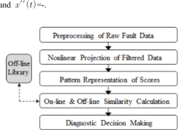
Fig. 1. Overall framework
As shown in the proposed framework of Fig. 1 raw fault data is preprocessed or filtered to eliminate the unuseful portion of the data when a fault is detected.
Then the filtered data is projected onto nonlinear KFDA to obtain the scores for the fault data. And the extraction of fault pattern is performed, which is followed by comparing the extracted fault pattern with the existing fault patterns. Finally diagnostic decision can be made at that time sequence, and this process can be repeated for the next time intervals.
The fault pattern vector at the jth time x(j) is given by x(j)=[x1,x2, ... ,xj]T, where xj is a fault element vector xj=[x1i,x2i, ... ,x7i]T. Each of xj should be 0 or 1, and the value of 1 represents the presence of the seven basic triangular components. For example, suppose that the fault patterns are observed as a sequence of 1-2-3 (i.e., constant, linear increase, and linear decrease).
The x1 at the 1st sequence is given: x1=[1,0,0,0,0,0,0]T. For others x2=[0,1,0,0,0,0,0]T and x3=[0,0,1,0,0,0,0]T. Overall, x(3)=[1000000 0100000 0010000]T. On-line fault pattern vector x(j) can be compared with off-line fault library vectors yk(j) obtained from training data.
For this purpose, the distance between x(j) and the kth
yk(j) is calculated ∥ ∥ Finally, a diagnosis decision at the jth time is made based on the similarity measure, which is given by
3. Results
The diagnosis performance of the proposed method is demonstrated, in which simulation data obtained from the Tennessee Eastman process is utilized. This process is a common test-bed for continuous processes[10]. It consists of five major units: reactor, condenser, separator, compressor, and stripper. The reactions in the reactor are as follows:
A+C+D→G, A+C+E→H, and A+E→F+3D→2F.
This process produces two products (i.e., noted by G and H) from four reactants (A, C, D, and E) with inert (B) and byproduct (F). A total of 53 process variables are measured on-line. The gaseous reactants are fed to the reactor, where the liquid products G and H are formed.
In this case study fifteen different faults are tested for a performance comparison purpose, which is listed in Table 1.
Fig. 2. A simulation process diagram
For each of the fifteen process faults training and test data sets were generated and used as fault library
and on-line fault data, respectively. As an example, Fig. 3 shows control charts for the training data of the process fault 1. In these charts, an out-of-control signal is detected around the time interval 600. These error signal fluctuated quickly up and down during that time intervals.
Table 1. List of process faults
Fault Description
1 A/C feed ratio, B composition constant 2 B composition, A/C ratio constant 3 D feed temperature
4 Reactor cooling water inlet temperature 5 Condenser cooling water inlet temperature 6 A feed loss
7 C header pressure loss 8 A/B/C feed composition 9 D feed temperature 10 C feed temperature
11 Reactor cooling water inlet temperature 12 Condenser cooling water inlet temperature 13 Reaction kinetics
14 Reactor cooling water valve 15 Condenser cooling water valve
The charts on other process faults, though not shown here, showed a similar behavior. After the detection of the fault it is necessary to find the on-line fault pattern.
Similarly the on-line fault patterns for the next sequences can be determined.
Fig. 3. A control chart for process fault 1
The on-line pattern vector at the specific time should be compared with the existing fault library patterns. Finally the similarity values are obtained for
each cause candidate, and a diagnostic decision can be made to select as the assignable cause the cause candidate with the highest similarity. Table 2 shows the results of diagnostic success rate for the simulation process. These values of the success rate are obtained from the proposed scheme that utilizes filtering and fault pattern matching of KFDA scores. In Table 2 the success rate (%) of the fifteen faults are listed for the training and test data sets. When the true cause of the fault is 1, for example, the success rates for the training and test data sets of the fault 1 are 98.6% and 96.9%. It means that only 1.4% and 3.1% of the diagnostic decision are incorrect for the training and test data, respectively. It should be also noted that the success rates for the training data are higher than those of the test data. Overall, the proposed scheme produced reliable diagnostic results for the data sets: 94.7%
average success rate for the training data and 92.5% for the test data.
Table 2. Results in success rate No. Success Rate (%)
No. Success Rate (%)
Training Test Training Test
1 98.6 96.9 9 88.3 86.2
2 97.1 96.0 10 89.5 87.0
3 99.0 98.2 11 92.0 89.6
4 98.3 96.7 12 88.1 85.4
5 98.6 96.4 13 93.3 90.9
6 98.8 97.1 14 92.9 90.3
7 99.4 96.3 15 93.6 89.7
8 92.6 90.5 Avg. 94.7 92.5
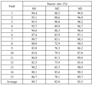
As shown in Table 3, the results of the success rates for the same test data were obtained from two different methods of “M1” and “M2”. Here “M3” indicates the proposed method, and the success rates of Table 1 are reproduced in Table 3. For a comparison purpose,
“M1” is different with “M3” in that it did not filter the raw data prior to performing KFDA and fault pattern matching. Similarly “M2” did OSC filtering and pattern matching, but utilized linear discriminant analysis instead of KFDA. As shown in Table 3 M3 of the proposed diagnostic scheme produced the best success rates for the fifteen test faults of this work. In
terms of average success rate, furthermore, M3 yielded the highest average value of 92.5% whilst M1 and M2 is 88.7% and 82.8%, respectively. Thus it can be said that the proposed diagnostic scheme outperforms the tested methods with linear and no filtering schemes. It should be also noted that the performance of M1 is better than that of M2 in all the test faults. The effect of selecting linear or nonlinear methods is more critical in the results than the preprocessing of raw data. It may be due to the fact that nonlinear data cannot be modeled well by linear methods.
Table 3. Results of three schemes
Fault Sucess rate (%)
M1 M2 M3
1 94.4 88.2 96.9
2 93.1 88.6 96.0
3 95.5 90.8 98.2
4 93.7 89.9 96.7
5 94.6 86.3 96.4
6 87.4 83.9 97.1
7 90.7 83.1 96.3
8 80.0 72.9 90.5
9 83.8 76.3 86.2
10 83.8 79.5 87.0
11 86.0 81.3 89.6
12 82.5 73.9 85.4
13 90.2 85.3 90.9
14 88.1 83.6 90.3
15 86.7 78.1 89.7
Average 88.7 82.8 92.5
4. Conclusion
In this work the efficient representation and matching of fault patterns in reduced spaces is demonstrated using simulation process data. It does not depend on certain mathematical models or expert’s knowledge. Only multivariate process data is required to make a diagnostic decision. In addition, the preprocessing of raw process data was performed in order to improve pattern matching results. The diagnosis results were obtained and tested from various diagnosis schemes. Resultantly it turned out that the use of filtering and nonlinear methods produced better
performance of diagnosis success rate than others. The proposed scheme is easy to implement because it requires only historical and on-line measurement data of processes.
References
[1] S. J. Qin, "Survey on data-driven industrial process monitoring and diagnosis", Annual Reviews in Control, 36, pp. 220-234, 2012.
DOI: https://doi.org/10.1016/j.arcontrol.2012.09.004 [2] S. Bersimis, S. Psarakis, J. Panaretos, "Multivariate
statistical process control charts: an overview", Quality and Reliability Engineering International, vol. 23, no. 5, pp. 517–543, 2007.
DOI: https://doi.org/10.1002/qre.829
[3] Z. Ge, Z. Song, F. Gao, “Review of recent research on data-based process monitoring”, Industrial and Engineering Chemistry Research, 52, pp. 3543-3562, 2013.
DOI: https://doi.org/10.1021/ie302069q
[4] L. Eriksson, J. Trygg, S. Wold, “A chemometrics toolbox based on projections and latent variables”, Journal of Chemometrics, 28, pp. 332-346, 2014.
DOI: https://doi.org/10.1002/cem.2581
[5] S. J. Qin, "Statistical process monitoring: basics and beyond", Journal of Chemometrics, 17, pp. 480–502, 2003.
DOI: https://doi.org/10.1002/cem.800
[6] L. H. Chiang, E. L. Russell, R. D. Braatz, "Fault diagnosis in chemical processes using Fisher discriminant analysis, discriminant partial least squares, and principal component analysis", Chemometrics and Intelligent Laboratory Systems, 50, pp. 243-252, 2000.
DOI: https://doi.org/10.1016/S0169-7439(99)00061-1 [7] G. Baudat, F. Anouar, Generalized discriminant analysis
using a kernel approach, Neural Computation, 12, pp.
2385-2404, 2000.
DOI: https://doi.org/10.1162/089976600300014980 [8] J. A. Westerhuis, S. Jong, A. K. Smilde, “Direct
orthogonal signal correction”, Chemometrics and Intelligent Laboratory Systems, 56, pp. 13-25, 2001.
DOI: https://doi.org/10.1016/S0169-7439(01)00102-2 [9] J. T.-Y. Cheung, G. Stephanopoulos, “Representation of
process trends-part I. a formal representation framework,” Computers and Chemical Engineering, vol.
14, pp. 495-510, 1990.
DOI: https://doi.org/10.1016/0098-1354(90)87023-I [10] J. J. Downs, E. F. Vogel, “A plant-wide industrial
process problem,” Computers and Chemical Engineering, vol. 7, pp. 245-255, 1993.
DOI: https://doi.org/10.1016/0098-1354(93)80018-I
Hyun-Woo Cho [Regular member]
•Aug. 2003 : POSTECH., Industrial Eng., PhD
•Aug. 2003∼Aug. 2007 : GIT/UT, Research Associate
•Sep. 2007 ∼ Feb. 2011 : SEC, Senior Engineer
•Mar. 2011 ∼ Current : Daegu Univ., Dept. of Industrial. &
Management Eng., Professor
<Research Interests>
Intelligent Process Monitoring, Data Mining