난류 파이프 유동 내 물질전달에 대한 레이놀즈 수 영향:
PartⅡ. 순간농도장, 고차 난류통계치 및 물질전달수지
강 창 우, 양 경 수*
인하대학교 기계공학부
R EYNOLDS N UMBER E FFECTS ON M ASS T RANSFER IN T URBULENT P IPE F LOW:
P ART II . I NSTANTANEOUS C ONCENTRATION F IELD, H IGHER- O RDER S TATISTICS AND M ASS T RANSFER B UDGETS
Changwoo Kang and Kyung-Soo Yang
*Dept. of Mechanical Engineering, Inha Univ.
Large Eddy Simulation(LES) of turbulent mass transfer in fully developed turbulent pipe flow has been performed to study the effect of Reynolds number on the concentration fields at
=180, 395, 590 based on friction velocity and pipe radius. Dynamic subgrid-scale models for the turbulent subgrid-scale stresses and mass fluxes were employed to close the governing equations. Fully developed turbulent pipe flows with constant mass flux imposed at the wall are studied for Sc=0.71. The mean concentration profiles and turbulent intensities obtained from the present LES are in good agreement with the previous numerical and experimental results currently available.
The effects of Reynolds number on the turbulent mass transfer are identified in the higher-order statistics(Skewness and Flatness factor) and instantaneous concentration fields. The budgets of turbulent mass fluxes and concentration variance were computed and analyzed to elucidate the effect of Reynolds number on turbulent mass transfer.
Furthermore, to understand the correlation between near-wall turbulence structure and concentration fluctuation, we present an octant analysis in the vicinity of the pipe wall.
Key Words :
대와류모사(Large Eddy Simulation), 난류 파이프 유동(Turbulent pipe flow), 물질전달(Mass transfer)Received: March 26, 2012, Revised: August 6, 2012, Accepted: August 7, 2012.
* Corresponding author, E-mail: [email protected] DOI http://dx.doi.org/10.6112/kscfe.2012.17.3.059
Ⓒ KSCFE 2012
1.
서 론난류 파이프 유동에서의 난류물질전달에 관한 공학적 중요 성은 앞선 난류 파이프 유동 내 물질전달에 대한 레이놀즈 수 영향
(PartⅠ)에서 언급되었다.
앞선 연구에서는 레이놀즈 수 변화에 따른 평균 농도장,
농도섭동 및turbulent mass fluxes의 변화에 대하여 알아보았으며 ,
이번 연구에서는 레이 놀즈 수 변화가higher-order statistics(Skewness and Flatness)와
순간 농도장
,
농도variance
및turbulent mass flux의 수지에 미
치는 영향에 대하여 알아보고자 한다.
파이프 유동에서의 농도섭동에 대한
Skewness와 Flatness에
대한 연구는 낮은 레이놀즈 수에 국한되었다. Piller[1]는
=180에서 DNS
계산을 통하여 농도섭동의Skewness와 Flatness
를 계산하였으며, Redjem-Saad et al.[2]은
=186에서 Prandtl
수( )의 변화에 따른 농도섭동의 Skewness와 Flatness를 계
산하였다 ≤ ≤ .
아직까지 더 높은 레이놀즈 수 에서Skewness와 Flatness에 대한 연구는 수행되지 않았다 .
농도
variance의 수지에 대한 연구는 Satake and Kunugi[3]
와
Piller[1]에 의하여 낮은 레이놀즈 수에서 수행되었으며,
turbulent mass fluxes의 수지에 대한 연구도 Satake and
Kunugi[3]에 의하여 낮은 레이놀즈 수(
=180)에서 수행되
었다. 따라서 더 높은 레이놀즈 수에서의 농도variance
및turbulent mass fluxes의 수지에 대한 연구가 필요하다.
따라서 본 연구에서는 동아격자 모델(Dynamic Subgrid-scale
Model)을 적용한 LES
기법을 이용하여
의 변화가 난류 파이프 유동 내 물질전달에 미치는 영향에 대한 두 번째 연 구로서Skewness, Flatness, 농도 variance
및turbulent mass fluxes의 수지의 변화에 대한 연구를 수행하였다 . LES가 수행
된
범위는180, 395, 590이며 로 고
정하였다. 여기서
는 관내 금속 벽면의 부식을 유발하는 산소 이온의 확산을 스칼라로 간주하여 고려되었다.
인 경우에 대하여 기존의 실험 및 수치해석 연구 결과들과 검증하였으며,
기존에 수행되지 않았던
에서의 계산을 통해
변화에 따른 난류 농도장의 통계치들의 변 화를 관찰하였다. 또한octant analysis를 통해 벽면 근처에서
의 난류 구조와 농도 섭동 사이의 상관관계를 살펴보았다.
2.
수치해석 기법본 연구에서 사용된
LES
기법을 위해 여과된 지배방정식 은 다음과 같다[4].
∇· (1)
∇· ∇ ∇·
∇
∇
(2)
∇· ∇·
∇ (3)
여기서
′ ′ 는 box filter를 사용하여
여과된 속도성분,
몰농도이고
와
는 각각total viscosity (
)와 total diffusivity(
)를 나타낸다 .
는 여과된 압력성분과 아격자 레이놀즈 응력의isotropic
성분 의 합
이다[4]. 아격자 레이놀즈 응력과 아격 자 농도 확산항은Germano et al.[5]과 Cabot and Moin[6]에 의
해 제시된 동아격자모델(Dynamic Subgrid-scale Model)을 이용
하여 다음과 같이 모델링되어지며,
(4)
∇ (5)
(eddy viscosity)와
(molecular diffusivity)는 다음과 같은 방
법으로dynamic
하게 계산된다.
∆
,
(6)
∆
(7)
∆ ∆
(8)
∆
,
(9)
∆
(10)
∆ ∆
∇
∇ (11)
여기서
,
는strain rate tensor, ∆
는filter width이며
∆
로 정의된다.
위의 지배방정식들은 논문
Part
Ⅰ에서와 같은 방법으로 차분되었다[7,8].
자세한 수치해석 기법은 논문Part
Ⅰ을 참고 하기 바란다.
본 연구에서 수행된 원형 직관의 형상,
유동장 및 농도장의 경계조건,
계산에 사용된 격자수 및 크기는 논문Part
Ⅰ과 동일하다.
그리고 고차의 난류 통계치를 계산하기 위하여
의100개의 sample로 축방향과 회전방향에
대하여 평균하였다.3.
결 과3.1 Skewness and Flatness of the concentration fluctuation Fig. 1과 Fig. 2는 각각
변화에 따른 농도섭동의Skewness
′
와Flatness
′
를 보여준다. 농도섭동의Skewness와 Flatness는 다음과 같이 정의되며 ,
′
〈
′
〉〈
′
〉, ′
〈
′
〉〈
′
〉(12)
Gaussian distribution은 각각 0과 3이다.
모든
에 대해서 벽면으로 근접함(
)에 따라 Skewness와 Flatness는 급
격히 증가하는 경향을 보이며, 중심부로 향할수록Gaussian distribution로 수렴한다 .
이는 벽면 근처에서의 농도섭동은 비 대칭적이고 간헐적인 특성을 갖는 것을 의미하고,
파이프의 중심부에서는homogeneous
특성을 갖는 것을 의미한다.
=180인 경우 벽면에서 ′ ≃ , ′ ≃
로Redjem
-Saad et al.[2]의 DNS
결과( ′ ≃ , ′ ≃ )보다
over-predict
되었다.
이는 난류 모델과 격자해상도의 영향으로 생각되어진다.y
+S( c' )
0 20 40 60 80 100
0 1 2
Reτ= 180 Reτ= 395 Reτ= 590
Fig. 1 Skewness factor of concentration fluctuation in the near-wall region
y
+F( c' )
0 20 40 60 80 100
0 2 4 6 8 10 12
Reτ= 180 Reτ= 395 Reτ= 590
Fig. 2 Flatness factor of concentration fluctuation in the near-wall region
3.2 Mass transfer budgets
LES
기법이 적용된Navier-Stokes
방정식과 농도 수송방정 식으로부터 유도된subgrid-scale
농도 확산항이 포함된 농도variance ,
〈′′
〉
와 난류mass flux의 수송방정식은
각각 다음과 같다.
〈
′′〉
〈
′〉
〈
′′〉
〈
′
′
〉
〈
〉 (13)
〈
′′〉
〈
′′〉
(14)
〈
′′〉
〈
′′〉
〈
′′′〉
〈
′′〉
〈
′′〉
〈
′ ′
〉
〈
′′
〉
〈
′ ′
〉
〈
′
′
〉
〈
〉
〈
〉
+ + + + + + + + + + + + + + + ++ + ++ ++ + + + ++ + ++ ++ ++ ++ ++ + + ++ ++ ++ ++ ++ ++ ++ + + + + +
y
+Lo ss G ai n
0 50 100 150
-0.2 -0.1 0 0.1 0.2
Production Turbulent transport Molecular diffusion Dissipation Satake and Kunugi(DNS) +
(a)
+ + ++ + + + + + + + + + + + + + + + ++ + + + + ++ ++ ++ ++ ++ ++ ++ ++ ++ ++ ++ ++ ++ ++ + + + +
y
+Lo ss G ai n
0 50 100 150
-0.2 -0.1 0 0.1 0.2
Production Turbulent transport Molecular diffusion Dissipation
Kawamura et al.(DNS, Channel) +
(b)
+ + + + + + + + + + + + + + + + + + + + + + + + + + + ++ + ++ ++ ++ ++ ++ + ++ ++ ++ ++ ++ ++ ++ ++ + + + +
y
+Lo ss G ai n
0 50 100 150
-0.2 -0.1 0 0.1 0.2
Production Turbulent transport Molecular diffusion Dissipation +
(c)
Fig. 3 Budgets of the concentration variance;
(a)
=180, (b)
=395, (c)
=590
여기서
,
는 각각 시간 및 공간 평균된 아격자 레이놀 즈 응력과 아격자 농도 확산항이다.본 연구에서는
subgrid-scale
농도 확산항은 제외한resolved
농도variance의 수지 (budget)를 계산하였다 .
본 연구에서와 같은 파이프 유동의 경우 축방향과 회전방향으로homogeneous
유 동으로 반경방향과 회전방향 평균속도(
)는 0이며,
회전 방향과 축방향으로의 평균값들의 미분 항들은 사라진다.
이와 같은 단순화가 적용된 자세한 각resolved
농도variance
및 난 류mass flux의 수지 식은 아래의 Appendix
Ⅰ에 나타내었다. 3.2.1 Budget for the concentration variance
Fig. 3은 각
에 대한resolved
농도variance(
)의 수지
를 나타낸 것이다.
인 경우Satake and Kunugi[3]의
DNS
결과와 비교하여 나타내었으며,
인 경우는Kawamura et al.[9]의 DNS
채널유동 결과와 비교하였다.+ + + + + + + + + + + + + + + + + ++ + + + + + + ++ + + ++ ++ ++ ++ ++ + ++ ++ ++ ++ ++ ++ ++ + + + +
+xxxxxxxxxxxxxxxxxxxxxxxxxxxxxxxxxxxxxxxxxxxxxxxxxxxxxxxxxxx
y
+Lo ss G ai n
0 50 100 150
-0.4 -0.2 0 0.2
0.4 ProductionTurbulent transport
Scalar pressure-gradient Viscous diffusion Molecular diffusion Dissipation Satake and Kunugi(DNS) +
x
(a)
+ + + + + + + + + + + + + + + + + + + + + + + + + ++ + ++ ++ ++ ++ ++ + ++ ++ ++ ++ ++ ++ ++ + + +
+xxxxxxxxxxxxxxxxxxxxxxxxxxxxxxxxxxxxxxxxxxxxxxxxxxxxxxxxx
y
+Lo ss G ai n
0 50 100 150
-0.4 -0.2 0 0.2
0.4 ProductionTurbulent transport
Scalar pressure-gradient Viscous diffusion Molecular diffusion Dissipation +
x
(b)
+ + + + + + + + + + + + + + + ++ + + + + + + + + + ++ + ++ ++ ++ ++ ++ ++ ++ ++ ++ ++ + ++ ++ ++ + + + +
+xxxxxxxxxxxxxxxxxxxxxxxxxxxxxxxxxxxxxxxxxxxxxxxxxxxxxxxxxxxxx
y
+Lo ss G ai n
0 50 100 150
-0.4 -0.2 0 0.2
0.4 ProductionTurbulent transport
Scalar pressure-gradient Viscous diffusion Molecular diffusion Dissipation +
x
(c)
Fig. 4 Budgets of the streamwise turbulent mass flux;
(a)
=180, (b)
=395, (c)
=590
인 경우는 비교 가능한 기존 연구결과가 존재하지 않으므로 본 연구에서의 계산 결과만 나타내었다. Fig. 3(a)에
서 보는 바와 같이
인 경우Satake and Kunugi[3]
의
DNS
결과와 비교하여 대체적으로 잘 일치하지만, 벽면 근 처에서 약간 차이를 보이는 것을 확인할 수 있다. Production
항은 ≤
≤ 에서
다소over-predict
되었으며,
≤
에서under-predict
되었다. Dissipation 항은 벽면으로
근접함에 따라under-predict된 경향을 보이지만 벽면 근처에
서는 다소over-predict되었다 .
이때 벽면에서는Dissipation
항 과Molecular diffusion 항이 균형을 이루며, Molecular diffusion
항도 벽면 근처에서 다소over-predict되었다 . Fig. 3(b)의
인 경우에도Kawamura et al.[9]의 DNS
채널유동 결과와 비교하였을 때 같은 경향을 보이는 것을 알 수 있다.
가 증가함에 따라 각 항들의 크기는
가 증가하는 것+ + + + + + + ++ ++ + + + + + ++ + + + + ++ + ++ ++ + ++ ++ + ++ ++ ++ ++ ++ + ++ ++ ++ + + + + + +
+xxxxxxxxxxxxxxxxxxxxxxxxxxxxxxxxxxxxxxxxxxxxxxxxxxxxxxxx x
x x
y
+Lo ss G ai n
0 50 100 150
-0.1 -0.05 0 0.05 0.1
Production Turbulent transport Scalar pressure-gradient Viscous diffusion Molecular diffusion Dissipation Satake and Kunugi(DNS) +
x
(a)
+ + + + + + + + + + + + + + + + + + ++ + + + ++ + ++ + ++ + + + ++ ++ ++ ++ ++ ++ ++ ++ ++ + + + +
+xxxxxxxxxxxxxxxxxxxxxxxxxxxxxxxxxxxxxxxxxxxxxxxxxxxxxx x
xx
y
+Lo ss G ai n
0 50 100 150
-0.1 -0.05 0 0.05 0.1
Production Turbulent transport Scalar pressure-gradient Viscous diffusion Molecular diffusion Dissipation
Kawamura et al.(DNS, Channel) +
x
(b)
+ + + + + + + + + + + + + + + + + + + + ++ + + + + ++ + ++ ++ ++ + + ++ ++ ++ ++ ++ ++ ++ ++ ++ + + + + +
+xxxxxxxxxxxxxxxxxxxxxxxxxxxxxxxxxxxxxxxxxxxxxxxxxxxxxxxxxx x
x x
y
+Lo ss G ai n
0 50 100 150
-0.1 -0.05 0 0.05 0.1
Production Turbulent transport Scalar pressure-gradient Viscous diffusion Molecular diffusion Dissipation +
x
(c)
Fig. 5 Budgets of the wall-normal turbulent mass flux;
(a)
=180, (b)
=395, (c)
=590
만큼 크게 변하지 않는다. 하지만
Dissipation
항은 다른 항들 에 비하여 벽면 근처에서의 크기가 좀 더 증가함을 확인할 수 있다.
또한
가 증가함에 따라 각 항들의peak
위치(
)는 점차 벽면으로 근접하였다 .
3.2.2 Budget for the streamwise mass flux
Fig. 4는 각
에 대한resolved
축방향 난류mass flux의
수지를 나타낸 것이다.
인 경우Satake and Kunugi[3]의 DNS
결과와 비교하여 나타내었다. Satake andKunugi[3]의 DNS
결과와 비교하여 대체적으로 잘 일치하지만resolved
농도variance(
)의 수지에서와 같이 벽면 근처에서
약간 차이를 보였다. Production 항은 ≤
≤
에서 다 소over-predict
되었으며, ≤
에서under-predict
되었다.Dissipation
항은 벽면으로 근접함에 따라under-predict된 경향
z
+r
+θ
0 250 500 750 1000
0 200 400 600
8 6 4 2 0 -2
c'+
(a)
z
+r
+θ
0 250 500 750 1000
0 200 400 600
10 8 6 4 2 0 -2 -4
uz'+
(b)
z
+r
+θ
0 250 500 750 1000
0 200 400 600
0.8 0.5 0.2 -0.1 -0.4
ur'+
(c)
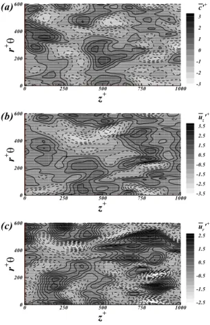
Fig. 6 Instantaneous resolved concentration and velocity fluctuations at
≃ for
; (a) concentration fluctuations, (b) axial velocity fluctuations, (c) radial velocity fluctuations. Dashed lines ; negative fluctuations, Solid lines ; positive fluctuations
을 보이지만 벽면 근처에서는 다소
over-predict되었다.
이때 벽면에서는Dissipation
항은Viscous diffusion, Molecular diffusion
항과 균형을 이루었다. Turbulent transport 항은 벽면
근처에서 다소over-predict되었으며,
벽면에서Production
항과Turbulent transport항은 0으로 수렴하였다.
가 증가함에 따 라 각 항들의peak에서의 크기는 다소 증가하였다.
특히Dissipation, Viscous diffusion 그리고 Molecular diffusion항의 크
기는 다른 항들에 비하여 좀 더 증가하였다. 또한Production
항과Turbulent transport 항의 크기가 peak가 되는 위치 (
)는
점차 벽면으로 근접하였다.3.2.3 Budget for the wall-normal mass flux
Fig. 5는 각
에 대한resolved
반경방향 난류mass flux
의 수지를 나타낸 것이다.
인 경우Satake and
z
+r
+θ
0 250 500 750 1000
0 200 400 600
3 2 1 0 -1 -2 -3
c'+
(a)
z
+r
+θ
0 250 500 750 1000
0 200 400 600
3.5 2.5 1.5 0.5 -0.5 -1.5 -2.5 -3.5
uz'+
(b)
z
+r
+θ
0 250 500 750 1000
0 200 400 600
2.5 1.5 0.5 -0.5 -1.5 -2.5
ur'+
(c)
Fig. 7 Instantaneous resolved concentration and velocity fluctuations at
≃ for
; (a) concentration fluctuations, (b) axial velocity fluctuations, (c) radial velocity fluctuations. Dashed lines ; negative fluctuations, Solid lines ; positive fluctuations
Kunugi[3]의 DNS
결과와 비교하여 나타내었으며,
인 경우는
Kawamura et al.[9]의 DNS
채널유동 결과와 비교하 였다. Fig. 5(a)에서
인 경우Satake and Kunugi[3]
의
DNS
결과와 비교하였을 때, Production 항과Scalar pressure-gradient
항이under-predict
되었다. 하지만 그 차이는 농도variance와 축방향 난류 mass flux의 수지에서의 차이보
다 작은 크기이다.
벽면 근처에서 반경방향 난류mass flux의
수지는 농도variance와 축방향 난류 mass flux의 수지와는 다
르게Production
항과scalar pressure-gradient 항이 지배적인 것
을 확인할 수 있다. Fig. 5(b)에서
인 경우에도
인 경우와 같은 경향을 보인다.
가 증가함에 따라Production, scalar pressure-gradient 그리고 Turbulent
transport
항의peak에서의 크기는 점차 증가하였으며,
위치(
)는 벽면 쪽으로 가까워진다 .
z' +u
z'
−u
r'
−u
r' +u
O
1O
2O
3O
4Negative scalar Outward Interaction Negative scalar
Ejection
Negative scalar Wallward Interaction
Negative scalar Sweep
< 0 ' c
z' +u
z'
−u
r'
−u
r' +u
O
5O
6O
7O
8Positive scalar Outward Interaction Positive scalar
Ejection
Positive scalar Wallward Interaction
Positive scalar Sweep
> 0 ' c
Fig. 8 Definition of Octants
3.3 Instantaneous concentration field
Fig. 6과 Fig. 7은
인 경우의 순간 유동장에서의 농도 및 속도섭동의 등고선을 나타낸 것이다.
여기서 실선은 양의 값을 나타내며,
점선은 음의 값을 나타낸다. Fig. 6에서 와 같이 벽면 근처에서의 농도 및 속도섭동의 등고선은 주유 동방향으로 가늘고 긴 형태의eddy
구조를 보인다. 농도섭동 은 반경방향 속도성분에 비하여 축방향 속도성분과 높은 상 관관계를 갖는 것을 확인할 수 있다. Fig. 7에서와 같이 파이 프의 중심부 근처에서는 농도섭동과 속도섭동은 낮은 상관관 계를 보이며, isotropic 형태의 구조를 보인다.
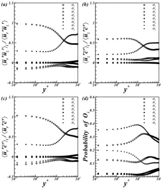
3.4 Octant analysis
농도장에서의 난류 구조를 파악하기 위해서
Octant analysis를
수행하였다[10]. Octant(
)는 속도섭동과 농도섭동의 부
호에 의하여Fig. 8에서와 같이 정의된다[10]. Fig. 9-11은 각
에 대한Reynolds shear stress, streamwise turbulent mass flux, wall-normal turbulent mass flux의 Octant analysis 결과와
각Octant
성분의probability를 나타낸 것이다.
Fig. 9(a), 10(a), 11(a)는 각
에 대한Reynolds shear stress의 Octant analysis 결과를 보여준다.
모든
에 대해서y
+〈u
r'u
z'〉
i/〈 u
r'u
z'〉
10-1 100 101 102
-0.5 0 0.5 1
1.5 O
O12 O3 O4 O5 O6 O7 O8
(a)
y
+〈u
z'c '〉
i/〈 u
z'c '〉
10-1 100 101 102
-0.5 0 0.5 1
1.5 O
O12 O3 O4 O5 O6 O7 O8
(b)
y
+〈u
r'c '〉
i/〈 u
r'c '〉
10-1 100 101 102
-0.5 0 0.5 1
1.5 O
O12 O3 O4 O5 O6 O7 O8
(c)
y
+P ro ba bility of O
i10-1 100 101 102
0 0.1 0.2 0.3 0.4 0.5
0.6 O
O12 O3 O4 O5 O6 O7 O8
(d)
![Fig. 3은 각 에 대한 resolved 농도 variance( )의 수지 를 나타낸 것이다. 인 경우 Satake and Kunugi[3]의 DNS 결과와 비교하여 나타내었으며 , 인 경우는 Kawamura et al.[9]의 DNS 채널유동 결과와 비교하였다](https://thumb-ap.123doks.com/thumbv2/123dokinfo/5522691.460270/3.808.429.733.111.632/나타낸-것이다-결과와-비교하여-나타내었으며-경우는-채널유동-비교하였다.webp)
![Fig. 4는 각 에 대한 resolved 축방향 난류 mass flux의 수지를 나타낸 것이다. 인 경우 Satake and Kunugi[3]의 DNS 결과와 비교하여 나타내었다](https://thumb-ap.123doks.com/thumbv2/123dokinfo/5522691.460270/4.808.432.732.110.618/resolved-축방향-수지를-나타낸-것이다-결과와-비교하여-나타내었다.webp)