Bayesian Multiple Comparison of Bivariate Exponential Populations based on Fractional Bayes Factor

(1)

2006, Vol. 17, No. 3, pp. 843 850 2006, Vol. 17, No. 3, pp. 843 850 2006, Vol. 17, No. 3, pp. 843 850 2006, Vol. 17, No. 3, pp. 843 850～～～～

Bayesian Multiple Comparison of Bivariate Bayesian Multiple Comparison of Bivariate Bayesian Multiple Comparison of Bivariate Bayesian Multiple Comparison of Bivariate Exponential Populations based on Fractional Bayes Exponential Populations based on Fractional BayesExponential Populations based on Fractional Bayes Exponential Populations based on Fractional Bayes

Factor Factor Factor Factor

Jang Sik Cho Jang Sik ChoJang Sik Cho

Jang Sik Cho¹⁾¹⁾¹⁾¹⁾ ․․․․ Kil Ho ChoKil Ho ChoKil Ho ChoKil Ho Cho²⁾²⁾²⁾²⁾ ․․․․ Seung Bae ChoiSeung Bae ChoiSeung Bae ChoiSeung Bae Choi³⁾³⁾³⁾³⁾

Abstract Abstract Abstract Abstract

In this paper, we consider the Bayesian multiple comparisons problem for K bivariate exponential populations to make inferences on the relationships among the parameters based on observations. And we suggest the Bayesian procedure based on fractional Bayes factor when noninformative priors are applied for the parameters. Also, we give a numerical examples to illustrate our procedure.

Keywords Keywords Keywords

Keywords : Bayesian multiple comparison, Fractional Bayes factor, Noninformative priors, Posterior probability

1. Introduction 1. Introduction 1. Introduction 1. Introduction

In many cases of two components system, the lifetimes of the components are assumed independent for convenience of computation. However it is more realistic to assume some form of dependence among components in many life testing situations. Let's consider a system which functions only as long as at least one of two identical or very similar components functions. Initially let the two components be independently on test with life distributions that are exponential with parameters _λ. Failure of one changes the life distribution of the other to

1) (Corresponding Author) Associate Professor, Department of Informational Statistics, Kyungsung University, Busan, 608-736, Korea.

E-Mail : [email protected]

2) Professor, Department of Statistics, Kyungpook National University, Daegu, 702-701, Korea

E-mail : [email protected]

3) Assistant Professor, Department of Information Statistics, Dongeui University, Busan, 614-714, Korea

E-mail : [email protected]

(2)

exponential with parameter _λζ > 0, where _ζ= 1 implies the independence of the two components lives. For _ζ > 1 the workload of the remaining component is increased, thereby decreasing the mean life. We call _ζ as dependence parameter. For this bivariate exponential model, Weier(1981) and Lee et.al.(1998) obtained Bayes estimators of parameters and reliability.

For testing equality of dependence parameters in two independent bivariate exponential populations, classical tests such as approximate test are widely used.

But the test of equality of dependence parameters more than three populations relies on likelihood ratio test statistic which is distributed as approximately χ² -distribution. And classical tests only decide whether the null hypothesis, commonly the equality of the parameters, will be rejected or not. When the null hypothesis is rejected, we don't know which hypothesis is best for describing the equality of parameters. But Bayesian approach to resolve the multiple comparisons problem selects the model with the highest posterior probability. And we can compute all the posterior probabilities of the hypotheses under consideration.

In this paper, we focus on Bayesian multiple comparisons for K bivariate exponential populations based on Bayes factor. In many cases, noninformative priors for the parameters are used. Since noninformative priors are typically improper, the priors are only up to arbitrary constants which affects the values of Bayes factors.

Berger and Pericchi(1996) introduced the intrinsic Bayes factor(IBF) using a data splitting idea, which would eliminate the arbitrariness of improper priors.

O'Hagan(1995) proposed the fractional Bayes factor(FBF) to remove the arbitrariness. These approaches have shown to be quite useful in several statistical areas. Cho(2006) proposed the Bayesian procedure for independence test based on FBF in bivariate exponentail model.

In this paper, we extend the results of Cho(2006) and consider Bayesian multiple comparisons for K bivariate exponential populations based on FBF. Also we propose the procedure for Bayesian multiple comparisons of dependence parameters based on FBF when improper priors are applied for the parameters. Finally, we give some numerical examples to illustrate our procedure.

2. Preliminaries 2. Preliminaries 2. Preliminaries 2. Preliminaries

Let M₁,⋯,M_N be models under consideration. And let random sample (XXXX,YYYY)=( (X₁,Y₁),⋯,(X_n,Y_n)) have probability density function f((xxxx,yyyy)∣θⁱ) under model M_i,i= 1,⋯,N. The parameter vectors θ_i are unknown. Let π_i(θ_i) be the prior distribution of model M_i^{, and let} p_i be the prior probabilities of model M_i. Then the posterior probability that the model M_i is true is given as

(3)

P(M_i_∣xxxx,yyyy)=(j^∑=1^N

p_j

p_i B_ji)^-1^,

where B_ij is the Bayes factor of model M_j ^{to model} M_i ^{defined by}

B_ji= m_j(xxxx,yyyy) m_i(xxxx,yyyy) =

⌠⌡_Θ

j

f(xxxx,yyyy_∣θ_j)π_j(θ_j)dθ_j

⌠⌡_Θ

i

f(xxxx,yyyy_∣θ_i)π_i(θ_i)dθ_i

. (1)

The B_ji interpreted as the comparative support of the data for the model j to i . The computation of B_ji needs specification of the prior distribution π_i(θ_i) and π_j(θ_j). Usually, one can use the noninformative prior which is improper. Let π^N_i be the noninformative prior for model M_i. Then the use of improper priors π^N_i(⋅) in (1) causes the B_ji to contain arbitrary constants.

To solve this problem, O'Hagan(1995) proposed the procedure for Bayesian testing and model selection problem based on FBF as follow. B_ij ^{based on} noninformative prior π^N_i(⋅) is given as

B^N_ji= m^N_j(xxxx,yyyy) m^N_i(xxxx,yyyy)=

⌠⌡_Θ

j

f(xxxx,yyyy_∣θ_j)π^N_j(θ_j)dθ_j

⌠⌡_Θ

i

f(xxxx,yyyy_∣θ_i)π^N_i(θ_i)dθ_i

. (2)

Hence the FBF of model M_j versus model M_i is given as

B^F_ji=q_j(b,xxxx,yyyy)

q_i(b,xxxx,yyyy), (3)

where q_i(b,xxxx,yyyy)=

⌠⌡_Θ

i

f_i(xxxx,yyyy_∣θ_i)π^N_i(θ_i)dθ_i

⌠⌡_Θ

i

f^b_i(xxxx,yyyy_∣θ_i)π^N_i(θ_i)dθ_i

and b specifies a fraction of the

likelihood which is to be used as a prior density. One frequently suggested choice is b = m/n, where m is the size of the minimal training sample.

Let's consider K populations with parameters Θ=(θ₁,θ₂,⋯,θ^K). Let

(XXXX_iiii,YYYY_iiii)=( (X_i₁,Y_i₁),⋯,(X_∈_i,Y_∈_i)) be a n_i×1 vector of independent observations on θ_i with density f(x_ij,y_ij_∣θ_i), i= 1,⋯,K, j= 1,⋯,n_i. Then the likelihood function for Θ given (XXXX,YYYY)=( (X₁,Y₁),⋯,(X_n,Y_n)) is

(4)

L(Θ∣xxxx,yyyy)=∏^K

i= 1∏

n_i

j=1f(x_ij,y_ij_∣θ_i). (4)

The multiple comparisons of K populations is to make inferences concerning relationships among the θ_i's based on (XXXX,YYYY).

Let Ω= { (θ₁,θ₂,⋯,θ^K): θ_i∈R, i= 1,2,⋯,K} be the K-dimensional parameter space. Equality and inequality relationships among the θ_i's induce statistical hypotheses such that subsets of Θ, i.e., M₁: Ω₁= {θ_i:θ₁= θ₂=⋯=θK}, M₁: Ω₁= { θ_i:θ₁≠θ₂=⋯= θ^K} and so on up to M_N: Ω_N= { θ_i:θ₁≠θ₂≠⋯≠θ^K} . The hypotheses M _r:Ω _r,r= 1,2,⋯,N^, ^are disjoint, and ∪^N_r_{= 1}Ω_r= Ω .

Each hypothesis can classified r(r= 1,⋯,K) distinct groups. Let θ^*₁,⋯,θ^*^r denote the set of distinct θ_i's, where r is the number of distinct elements in the vector Ω. We need to define the configuration notation.

Definition 1 Definition 1 Definition 1

Definition 1 (Configuration)(Configuration)(Configuration)(Configuration). The configuration S={S₁,⋯,S_K} determines a classification of θ into r distinct groups or clusters. Write K_j for the set of indices of parameters in group j, K _j= {i:S _i=j} . Let n_K

j= {n_i_∣i∈K_j} be the index set of observations and θ^*_j be the common parameter value for K_j^.

There is a one to one correspondence between hypotheses and configurations.

Therefore the Bayes factor for multiple comparisons can easily compute by this configuration notation.

Suppose that a model is classified r distinct groups. Then the likelihood function is given by

L(^θ^*₁^,_⋯,θ^*r∣xxxx,yyyy)⁼ ∏

r

t=1 ∏

{i:i∈K_t}∏

n_i j=1

f(x_ij,y_ij_∣θ_t). (5) Since the noninformative prior for the model is π^N_r(θ^*₁,⋯,θ^*r), the FBF is given by

q(b,xxxx,yyyy)=

⌠⌡

∞ -∞⋯⌠

⌡

∞ -∞

L(^θ^*1,⋯,θ^*r∣xxxx,yyyy)_⋅π^Nr(^θ^*¹^,^⋯,θ^*^r)^d^θ^*¹^⋯^d^θ^*^r

⌠⌡

∞ -∞⋯⌠

⌡

∞ -∞

L^b(^θ^*1,⋯,θ^*r∣xxxx,yyyy)_⋅π^Nr(^θ^*¹^,^⋯,θ^*^r)^d^θ^*¹^⋯^d^θ^*^r^. ⁽⁶⁾

Thus if a model M_i is classified r_i distinct groups and a model M_j ^is classified r_j distinct groups then the FBF of M_j ^versus M_i is given by

(5)

B^F_ji=q_j(b,xxxx,yyyy) q_i(b,xxxx,yyyy),

where qi(b,xxxx,yyyy)=

⌠

⌡

∞ -∞⋯⌠

⌡

∞ -∞

L(^θ^*1,⋯,θ^*r_i∣xxxx,yyyy)⋅π^Nr_i(^θ^*¹^,^⋯,θ^*^rⁱ)^d^θ^*¹^⋯^d^θ^*^rⁱ

⌠⌡

∞ -∞⋯⌠

⌡

∞ -∞

L^b(^θ^*1,⋯,θ^*r_i∣xxxx,yyyy)⋅π^Nr_i(^θ^*¹^,^⋯,θ^*^rⁱ)^d^θ^*¹^⋯^d^θ^*^rⁱ^.

Hence the FBF for all comparisons can computed by equation (2). Using these FBF's, we can calculate the posterior probability for model M_i, i= 1,⋯,K^. Thus, we can select the hypothesis with highest posterior probability in Bayesian multiple comparisons based on FBF.

3. Bayesian Multiple Comparisons 3. Bayesian Multiple Comparisons 3. Bayesian Multiple Comparisons 3. Bayesian Multiple Comparisons

Let (XXXX_iiii,YYYY_iiii)=( (X_i₁,Y_i₁),⋯,(X_∈_i,Y_∈_i)) be a random sample from a bivariate exponential population with parameter vector θ_i= (λ_i,ζ_i). Then the joint probability density function for (X_ij,Y_ij) is given as

f(x_ij,y_ij:λ_i,ζ_i) = 2ζ_iλ²_iexp(-2λ_ix_ij-λ_iζ_iy_ij), x_ij,y_il>0, λ_i,ζ_i>0.

Suppose that a model M_i ^classified ^r ^distinct ^groups. ^Then ^the noninformative prior for (θ^*₁,⋯,θ^*r) is

π^N_r( θ^*₁,⋯,θ^*r)= 1

c ^{, 0 < θ}^*¹^{< ∞,}^⋯,0<θ^*^r^{< ∞ ,} ⁽⁷⁾ where c is a fixed constant.

And likelihood function is

L(θ^*₁,⋯,θ^*^r∣xxxx,yyyy)

=∏^r

t=1{⁽²^⋅λ²^t^⋅ζ^t⁾^∣^K^t^∣^⋅exp(^-_i_∈^∑_K_t_j^∑₌₁ⁿⁱ⁽²^⋅λⁱ^⋅^x^ij^+λⁱ^⋅ζⁱ^⋅^y^ij⁾)}^, ⁽⁸⁾

where ∣K_t∣ is the number of the set of indices K_t^. Then the element of the FBF is computed as follows;

⌠⌡

∞

0 ⋯⌠⌡₀^∞L(θ^*₁,⋯,θ^*r∣xxxx,yyyy)π^N_r(θ^*₁,⋯,θ^*r)dθ^*₁⋯dθ^*_r

=c_⋅∏^r

t= 1

Γ(∣K_t_{∣)⋅Γ(∣}K_t_∣+1)⋅(i∈^∑K_t∑

ni

j=1x_ij)^-^∣^K^t^∣^⋅(i∈^∑K_t∑

ni

j=1y_ij)^-^∣^K^t^{∣ -1}

(6)

and

⌠⌡

∞

0 ⋯⌠

⌡

∞

0 L^b(θ^*₁,⋯,θ^*r∣xxxx,yyyy)π^N_r(θ^*₁,⋯,θ^*r)dθ^*₁⋯dθ^*_r

=c_⋅∏

r t=1

Γ(b_⋅∣K_t_∣)⋅Γ(b_⋅∣K_t_∣+1)⋅(^bi∈^∑K_t∑

n_i j=1

x_ij)^-^b^⋅∣^K^t^∣^⋅(^bi∈^∑K_t∑

n_i j=1

y_ij)^-^b^⋅∣^K^t^∣-1^.

Hence, q(b,xxxx,yyyy) is given as

q(b,xxxx,yyyy)=∏

r t=1

Γ(∣K_t_{∣)⋅Γ(∣}K_t_∣+1)⋅(^bi^∑∈K_t∑

n_i j=1

x_ij)^b^⋅∣^K^t^∣^⋅(^bi∈^∑K_t∑

n_i j=1

y_ij)^b^⋅∣^K^t^∣+1

Γ(b_⋅∣K_t_∣)⋅Γ(b_⋅∣K_t_∣+1)⋅(i∈^∑K_t∑

n_i j=1

x_ij)^∣^K^t^∣^⋅(i^∑∈K_t∑

n_i j=1

y_ij)^∣^K^t^∣+1 ^. ⁽⁹⁾

Thus if a model M_i is classified r_i distinct groups and a model M_j ^is classified r_j distinct groups then the FBF of M_j ^versus M_i is given by

B^F_ji(xxxx,yyyy)=q_j(b,xxxx,yyyy) q_i(b,xxxx,yyyy), where

q_i(b,xxxx,yyyy)= ∏

r_i M_i:t=1

Γ(∣K_t_{∣)⋅Γ(∣}K_t_∣+1)⋅(^bi∈^∑K_t∑

n_i j=1

x_ij)^b^⋅∣^K^t^∣^⋅(^bi∈^∑K_t∑

n_i j=1

y_ij)^b^⋅∣^K^t^∣+1

Γ(b_⋅∣K_t_∣)⋅Γ(b_⋅∣K_t_∣+1)⋅(i^∑∈K_t∑

n_i j=1

x_ij)^∣^K^t^∣^⋅(i∈^∑K_t∑

n_i j=1

y_ij)^∣^K^t^∣+1

and

q_j(b,xxxx,yyyy)= ∏

r_j M_j:t=1

Γ(∣K_t_{∣)⋅Γ(∣}K_t_∣+1)⋅(^bi^∑∈K_t∑

n_i j=1

x_ij)^b^⋅∣^K^t^∣^⋅(^bi∈^∑K_t∑

n_i j=1

y_ij)^b^⋅∣^K^t^∣+1

Γ(b_⋅∣K_t_∣)⋅Γ(b_⋅∣K_t_∣+1)⋅(i^∑∈K_t∑

n_i j=1

x_ij)^∣^K^t^∣^⋅(i∈^∑K_t∑

n_i j=1

y_ij)^∣^K^t^∣+1 ^.

(10)

4. Numerical Examples 4. Numerical Examples 4. Numerical Examples 4. Numerical Examples

In this section, we use a numerical data to illustrate the multiple comparisons for the dependence parameters of bivariate exponential populations based on FBF.

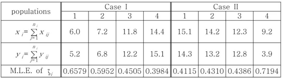
Here, we consider 4 bivariate exponential populations and sample size of 10 from each populations. In this paper, we consider multiple comparisons for two cases, so that true hypothesis are H _true:ζ₁= ζ₂≠ζ₃= ζ₄ for case I and

H _true:ζ₁= ζ₂= ζ₃≠ζ₄ for case II, respectively.

(7)

The observed summary statistics for each case are given as Table 1. And the numbers of possible hypothesis are 15 for each cases.

<Table 1> The observed summary statistics for each populations

populations Case I Case II

1 2 3 4 1 2 3 4

x_i= ∑

n_i

j= 1x_ij 6.0 7.2 11.8 14.4 15.1 14.2 12.3 9.2

y_i=∑

n_i j= 1

y_ij 5.2 6.8 12.2 15.1 14.3 13.2 12.8 3.9 M.L.E. of ζ_i 0.6579 0.5952 0.4505 0.3984 0.4115 0.4310 0.4386 0.7194

Table 2 gives the calculated posterior probabilities for all possible hypotheses based on FBF of case I and case II, respectively.

<Table 2> Calculated posterior probabilities for each cases based on FBF Hypothesis

Hypothesis Hypothesis

Hypothesis Case ICase ICase ICase I Case IICase IICase IICase II ζ₁= ζ₂= ζ₃= ζ₄ 0.0617 0.0460 ζ₁= ζ₂= ζ₃≠ζ₄ 0.1054 0.46830.46830.46830.4683 ζ₁= ζ₂= ζ₄≠ζ₃ 0.0111 0.0091 ζ₁= ζ₂≠ζ₃= ζ₄ 0.58650.58650.58650.5865 0.0429 ζ₁= ζ₂≠ζ₃≠ζ₄ 0.1014 0.0945 ζ₁= ζ₃= ζ₄≠ζ₂ 0.0102 0.0134 ζ₁= ζ₃≠ζ₂= ζ₄ 0.0077 0.0281 ζ₁= ζ₃≠ζ₂≠ζ₄ 0.0069 0.1035 ζ₁= ζ₄≠ζ₂= ζ₃ 0.0055 0.0181 ζ₁= ζ₄≠ζ₂≠ζ₃ 0.0013 0.0028 ζ₁≠ζ₂= ζ₃= ζ₄ 0.0433 0.0216 ζ₁≠ζ₂= ζ₃≠ζ₄ 0.0202 0.1196 ζ₁≠ζ₂= ζ₄≠ζ₃ 0.0054 0.0050 ζ₁≠ζ₂≠ζ₃= ζ₄ 0.0284 0.0084 ζ₁≠ζ₂≠ζ₃≠ζ₄ 0.0049 0.0186

For case I, it is evident that the hypotheses for ζ₁= ζ₂≠ζ₃= ζ₄ has the most large posterior probabilities 0.5865. This suggests that the data lend

(8)

greatest support to equalities for ζ₁=ζ₂ and ζ₃=ζ₄ being different from the others. Thus this example shows good performance of the Bayesian multiple comparisons method based on FBF.

For case II, it is evident that the hypotheses for ζ₁= ζ₂= ζ₃≠ζ₄ has the most large posterior probabilities 0.4683. This suggests that the data lend greatest support to equalities for ζ₁= ζ₂= ζ₃ and ζ₄ being different from the others. Also this example shows good performance of the Bayesian multiple comparisons method based on FBF.

Up to this point, we have considered the problem of developing a Bayesian multiple comparisons for dependence parameter in K bivariate exponential populations. Extension of the above approach to the multiple comparison problems for the another population is straightforward. The research topics pertaining to the extension of the method and the examination of its performance are worthy to study and are left as a future subject of research.

References References References References

1. Ali, M.M., Cho, J.S. and Begum, M.(2005), Nonparametric Bayesian Multiple Comparisons for Geometric Populations, Journal of the Korean Data & Information Science Society, Vol. 16(4), 1129-1140.

2. Berge, C.(1971), Principle of Combinatorics , New York: Academic Press.

3. Berger, J. O. and Pericchi, L. R.(1996), The Intrinsic Bayes Factor for Model Selection and Prediction, Journal of the American Statistical Association, 91, 109-122.

4. Consonni, G. and Veronese, P.(1995), A Bayesian Method for Combining Results from Several Binomial Experiments, Journal of the American Statistical Association, 90, 935-944.

5. Fienberg, S. E.(1980). The Analysis of Cross-Classified Categrical Data, Cambridge, MA: The MIT Press.

6. Lee, I.S., Cho, J.S., Kang, S.G. and Ko, J.H.(1998), Bayes Computations for the Reliability in a Bivariate Expnential Model, The Korean

Communications in Statistics, 5(1), 145-153.

7. O' Hagan, A.(1995), Fractional Bayes Factors for Model Comparison(with discussion), Journal of Royal Statistical Society, 56, 99-118.

[ received date : Apr. 2006, accepted date : May. 2006 ]