Value at Risk Forecasting Based on Quantile Regression for GARCH Models

Value at Risk Forecasting Based on Quantile Regression for GARCH Models

Sangyeol Lee

· Jungsik Noh

1

Department of Statistics, Seoul National University

2

Department of Statistics, Seoul National University

Abstract

Value-at-Risk(VaR) is an important part of risk management in the financial industry. This paper presents a VaR forecasting for financial time series based on the quantile regression for GARCH models recently developed by Lee and Noh (2009). The proposed VaR forecasting features the direct conditional quantile estimation for GARCH models that is well connected with the model parameters. Empirical performance is measured by several backtesting procedures, and is reported in comparison with existing methods using sample quantiles.

Keywords: Quantile regression, GARCH models, Value-at-Risk.

1. Introduction

Value-at-Risk(VaR) has been widely accepted as a prominent measure of market risk by financial institutions and their regulators. Although VaR is nothing but a quantile of random variable, various methodologies are developed to calculate VaR. Among them, the quantile regression approach has been popular since it directly models a particular quantile rather than the whole return distribution of a certain portfolio. Since the quantile is tightly linked to the volatility of time series, and since generalized autoregressive conditional heteroscedasticity(GARCH) models are proven to be effective to measure the volatility, many authors consider the estimation procedure for VaR via the quantile regression based on GARCH models. As a representative reference, we refer to Engle and Manganelli (2004) who provided a nonlinear dynamic quantile model for VaR. Recently, Lee and Noh (2009) developed a quantile regression estimation method for GARCH models and demonstrated that it can be readily applicable to estimating the direct conditional quantile for GARCH models to obtain an one-step-ahead VaR estimator. In this paper, we study the out-of-sample performance of the conditional quantile estimation based on Lee and Noh’s (2009) method.

For clarity, we define VaR as follows, which is according to Chernozhukov and Umantsev (2001).

Let r

denote the return of a portfolio over [t − 1, t). The 100(1 − τ)% conditional VaR for holding

2Corresponding author: Post-Doctoral Fellow, Department of Statistics, Seoul National University, Seoul 151-742, Korea. E-mail: [email protected]

period 1 at time t is defined as

VaR

(τ ) = inf{x ; P (r

≤ x|F

) ≥ τ}, (1.1) where F

denotes the information up to time t. We denote an one-step-ahead 100(1 − τ)% VaR estimate at time t by d VaR

(τ ). When we forecast daily VaR, we adopt the rolling scheme, that is, at time t, d VaR

(τ ) is calculated from the last T

observations of daily returns, {r

, . . . , r

}.

This paper is organized as follows. In Section 2, we briefly review the quantile regression for GARCH models. In Section 3, we describe the VaR forecasting procedure based on the quantile regression for GARCH models and other existing methods. In Section 4, we examine the methods of testing the adequacy of the VaR forecasts. In Section 5.1, we illustrate a real data analysis.

2. Quantile Regression for GARCH Models

In order to incorporate the heteroscedasticity of portfolio returns into the calculation of VaR, we consider the GARCH model:

{ ε

= √ h

η

,

h

= ω

+ α

ε

+ β

h

, (2.1) where ω

> 0, α

≥ 0, β

≥ 0 and η

are i.i.d. random variables with zero mean and unit variance. Further, we assume that α

+ β

< 1 which is the necessary and sufficient condition for the second-order stationarity of model (2.1).

To formulate the quantile regression problem for GARCH models, Lee and Noh (2009) adopted the reparametrization approach, addressed below, since under the model (2.1), the τ quantile of ε

conditional on the past observations up to time t − 1 is not identifiable. In this reparametrization, we set σ

= √

h

/ω

, u

= √

ω

η

and γ

= α

/ω

to reformulate model (2.1) as { ε

= σ

u

, u

∼ i.i.d. (0, ω

),

σ

= 1 + γ

ε

+ β

σ

, (2.2) where ω

> 0, γ

≥ 0, β

≥ 0 and ω

γ

+ β

< 1. Let F

(τ ) be the τ quantile of u

for 0 < τ < 1.

Under the reparametrized GARCH(1, 1) model (2.2), the τ quantile of ε

conditional on F

is given by

Q

(θ

(τ ) |F

) := inf {x; P (ε

≤ x|F

) ≥ τ}

= F

(τ )σ

= F

(τ ) (

1 + γ

ε

+ β

σ

)

,

(2.3)

where we consider a new parameter ξ

(τ ) := F

(τ ) and denote the true parameter value by θ

(τ )

= (ξ

(τ ), γ

, β

).

Now, we can define the quantile regression estimator for the model (2.2). The parameter vector is denoted by θ

= (ξ, γ, β) and belongs to a compact parameter space

Θ

(ω

) = {

θ ∈ R

; |ξ| ≤ ξ

, ω

γ + β ≤ 1 − κ, γ, β ≥ 0 }

, (2.4)

where ξ

(possibly large enough) and κ (possibly small enough) are given positive real numbers. We

assume the true parameter value θ

(τ ) is an interior point of Θ

(ω

), which ensures the second-order

stationarity of the model (2.2). Suppose that ε

, ε

, . . . , ε

are observations from a GARCH(1, 1) process. For t ≥ 1, we define eσ

(γ, β) recursively by using the equation

eσ

(γ, β) = 1 + γε

+ β eσ

(γ, β), (2.5) where the initial value can be chosen as eσ

(γ, β) = 1. In view of (2.3), we denote the initialized conditional quantile function by

Q e

(θ|F

) = ξeσ

(γ, β)

and define the τ quantile regression estimator as any solution b θ

(τ )

= ( ˆ ξ

(τ ), ˆ γ

(τ ), ˆ β

(τ )) of bθ

(τ ) = argmin

θ∈Θκ( ˆω_n)

1 n

∑

ρ

(

ε

− e Q

(θ|F

) )

, (2.6)

where ρ

(x) = τ x

+ (1 − τ)x

, x

= max {x, 0} and x

= − min{x, 0}. Note that the domain for minimization is Θ

(ˆ ω

), where ˆ ω

is a consistent estimator of ω

, instead of the parameter space Θ

(ω

), since ω

is unknown. The following asymptotic property of b θ

(τ ) was proved by Lee and Noh (2009).

Theorem 2.1. Under some regularity conditions, for 0 < τ < 1 and ξ

(τ ) ̸= 0, bθ

(τ ) is strongly consistent and √

n(b θ

(τ ) − θ

(τ )) is asymptotically normal.

Remark 2.1. Note that for τ

such that ξ

(τ

) = 0, the τ

conditional quantile function in (2.3) equals to 0. Thus, the τ

quantile regression problem for GARCH models is ill posed in that case (cf. Remark 3.3 of Lee and Noh (2009)).

Since τ conditional quantile of ε

given F

is Q

(θ

(τ )|F

) = ξ

(τ )(1 + γ

ε

+ β

σ

)

, the VaR estimate for ε

conditional on the observations up to time t − 1 can be defined as

V ˆ

(τ ) := ˆ ξ

(τ )ˆ σ

= ˆ ξ

(τ ) (

1 + ˆ γ

(τ )ε

+ ˆ β

(τ )ˆ σ

)

2

, (2.7)

where ˆ σ

= eσ

(ˆ γ

(τ ), ˆ β

(τ )).

It is noteworthy that the proposed VaR (2.7) is essentially identical to the conditional autoregres- sive value at risk(CAViaR) with the indirect GARCH(1, 1) specification, proposed by Engle and Manganelli (2004), although some differences exist in their formula. Following their notation, the indirect GARCH(1, 1) specification is given by

VaR

(β) = (

β

+ β

VaR

(β) + β

ε

)

,

and the conditional VaR at time t − 1 is given by −VaR

( ˆ β) where β = argmin ˆ

β

1 n

∑

ρ

(ε

+ VaR

(β)) . Since for ξ < 0,

Q e

(θ |F

) = ( −1) (

ξ

+ β e Q

(θ |F

) + ξ

γε

)

,

due to (2.6) and (2.7), it can be seen that −VaR

( ˆ β) of Engle and Manganelli (2004) is the same

as ˆ V

(τ ) in (2.7).

3. VaR Forecasting

Suppose we are given time series of portfolio returns {r

; 1 ≤ t ≤ T }, where T denotes the length of the estimation period. Here, we consider the following AR(1)-GARCH(1, 1) model:

r

= a

+ a

r

+ ε

,

where a

∈ R, |a

| < 1 and {ε

} follows GARCH(1, 1) in (2.1) or (2.2).

Our interest is to forecast the one-step-ahead 100(1 − τ)% conditional VaR at time T , VaR

(τ ) in (1.1). The following procedure leads to a one-step-ahead VaR forecast based on the quantile regression for GARCH models. First, we estimate (a

, a

) by quasi maximum likelihood(QML) estimator and obtain AR residuals

ˆ

ε

= r

− ˆa

− ˆa

r

,

for t = 1, 2, . . . , T . Based on these residuals, following the method in Section 2, we can obtain τ quantile regression estimator ( ˆ ξ(τ ), ˆ γ(τ ), ˆ β(τ )) for the reparametrized GARCH model. Then, our proposed VaR is given by

VaR d

(τ ) = ˆ a

+ ˆ a

r

+ ˆ ξ(τ )ˆ σ

,

where ˆ σ

= eσ

(ˆ γ(τ ), ˆ β(τ )) in (2.5). We refer to this procedure as the QR method in Section 5.1.

To compare this VaR forecast, we take account of the two existing methods. The first one is based on Gaussian QML estimates and sample quantile of residuals. By using the above AR residuals {ˆε

}, we can obtain QML estimate (ˆω, ˆα, ˆ β), of which properties are well established in the literature (see, e.g., Francq and Zako¨ıan, 2004), and AR-GARCH residuals

ˆ η

= √ ε ˆ

ˆ h

,

where ˆ h

, t = 1, 2, . . . , T , are defined recursively by using ˆ h

= ˆ ω + ˆ αˆ ε

+ ˆ βˆ h

and an appropriate initial value for ˆ h

. Then, one possible VaR forecast is given by

VaR d

(τ ) = ˆ a

+ ˆ a

r

+ ˆ F

(τ )

√ ˆ h

,

where ˆ F

(τ ) is a τ sample quantile of {ˆη

; 1 ≤ t ≤ T }. We refer to this procedure as the QML method in Section 5.1. This VaR forecast may be regarded as a variant of the one proposed by Hull and White (1998).

The second one is the historical simulation method which has been used practically by financial institutions. The historical simulation VaR is simply the unconditional sample quantile of the past T observations, which is denoted by

VaR d

(τ ) = ˆ F

(τ ).

Remark 3.1. The VaR forecasts d VaR

(τ ) and d VaR

(τ ), based on ARMA-GARCH models

with general orders, can be also obtained in a similar fashion. However, conditional mean modeling

with higher orders does not strongly affect the result, so in our empirical study, we only consider

the AR(1) modeling for all return series.

4. Backtesting Measures

In the VaR framework, it is important to assess the quality of VaR estimates—a procedure known as backtesting. So far, various backtesting measures have been proposed in the literature. In this study, we consider the four tests addressed below which are widely used or recently developed (cf.

Berkowitz et al., 2009; Hartz et al., 2006; Lee and Lee, 2010).

Suppose we observe portfolio returns r

and have their one-step-ahead 100(1 − τ)% VaR forecasts { d VaR

(τ ) }, each of which is calculated at time t−1. We define the sequence indicating the presence or absence of VaR violations as {I

}

= {I(r

< d VaR

(τ )) }

. Here, {t; 1 ≤ t ≤ T } indicates the forecasting period. For correct VaR models, the violation I

are anticipated to be i.i.d. Bernoulli(τ ) random variables.

Note that a fundamental requirement for quantile estimators is that the proportion of observations falling below the τ quantile estimator should be τ . The Kupiec (1995) test is well known to satisfy this requirement and also as an unconditional coverage test. Note that the likelihood value under the null hypothesis, in which the probability equals to τ , is

L(τ ) =

∏

(1 − τ)

τ

= (1 − τ)

τ

,

where T

= ∑

t=1

I

means the number of violations and T

= T − T

. We denote the coverage rate by ˆ p = T

/T . In fact, the Kupiec test is a likelihood ratio(LR) test of the form

LR

= −2 log [ L(τ )

L(ˆ p) ]

,

which is asymptotically distributed as χ

(chi-square distribution with 1 degree of freedom). To assess the deviation of the coverage rate ˆ p from τ , we use the p-value P

= 1 − F

(LR

).

Along with the Kupiec test, Christoffersen’s (1998) conditional coverage test is also a well established joint test for coverage and independence, namely, it tests the hypotheses:

H

: I

’s are i.i.d. Bernoulli(τ ),

H

: I

’s are first order Markov sequence with the state space {0, 1}.

Let p

= Pr (I

= j | I

= i) be the transition probability from state i to j for i, j = 0, 1. Denote by T

the number of observations with j following i. The observed probabilities are given by

ˆ

p

= T

T

+ T

,

for i, j = 0, 1. Then, the LR test statistic and corresponding p-value are respectively LR

= −2 log

[ (1 − τ)

τ

ˆ

p

p ˆ

p ˆ

p ˆ

]

≈ χ

, P

= 1 − F

(LR

).

Since the de-meaned true violations {I(r

< VaR

(τ )) − τ} form a martingale difference sequence,

a natural testing strategy is to check whether or not the autocorrelations are negligible. From

this reasoning, one can consider employing the Ljung-Box(LB) test to test whether the first m

autocorrelations of {I

} are all zero (cf. Berkowitz et al., 2009). Denote the sample autocorrelation

at lag h by ˆ ρ(h). Then, the LB test statistic and corresponding p-value are given by

LB(m) = T (T + 2)

∑

ˆ ρ

(h)

T − h ≈ χ

, P

= 1 − F

(LB(m)).

In Section 5.1, LB(5) is utilized.

In fact, Engle and Manganelli (2004) also proposed a backtesting procedure called the dynamic quantile(DQ) test. In this study, we adopt a variant of the DQ test suggested by Berkowitz et al.

(2009). Note that by the definition of VaR in (1.1), for any X

adapted to F

, E [X

{I(r

< VaR

(τ )) − τ} |F

] = 0,

which means {I(r

< VaR

(τ )) − τ} must be uncorrelated with its own lagged values and with VaR

(τ ). In view of this, one can consider the autoregressive logistic model

P [I

= 1 |F

] = f (

α +

∑

β

I

+

∑

β

VaR d

(τ ) )

=: p

(θ) ,

where f (x) = (1 + exp(−x))

and θ = (α, β

, . . . , β

, β

, . . . , β

). The coefficients in the above equation are easily obtained using usual statistical packages supporting the generalized linear mod- els. Here, we consider to test the following hypotheses:

H

: α = log τ (1 − τ)

, β

= · · · = β

= 0, β

= · · · = β

= 0, H

: not H

.

Then, the LR test statistic and corresponding p-value are given by

LR

= −2 log



  (1 − τ)

τ

∏

( 1 − p

( θ ˆ ))

p

( θ ˆ )



  ≈ χ

, P

= 1 − F

(LR

).

In Section 5.1, we use P

with p = 2 and q = 1.

5. Empirical Analysis

5.1. Daily VaR forecasting for domestic financial time series

In this numerical study, all computations are performed with R software package. In particular, Rmetrics package is well known to be suitable to deal with ARMA-GARCH models (cf. W¨ urtz et al., 2002). For the quantile regression estimation for GARCH models, we use the Nelder-Mead simplex optimization algorithm by taking initial values as QML estimates.

In order to examine the performance of our one-step-ahead VaR forecasting method, we analyze the two Korean stock market indices, the KOSPI and KOSDAQ, Samsung Electronic Co. stock price, Korean Won/USD and Korean Won/Japanese Yen exchange rates. The stock market data taken from the Korea Exchange are daily observations of closing prices. The FX rates taken from the Korea Exchange Bank are daily quoted base rates at the last quotation time. We compute the daily returns as 100 times the difference of the log of the prices such as r

= 100 · (log p

− log p

).

The daily returns range from January 5, 2000 to December 24, 2009 for the three stock market

series, and from June 20, 2000 to December 24, 2009 for the two FX rates. The forecasting period

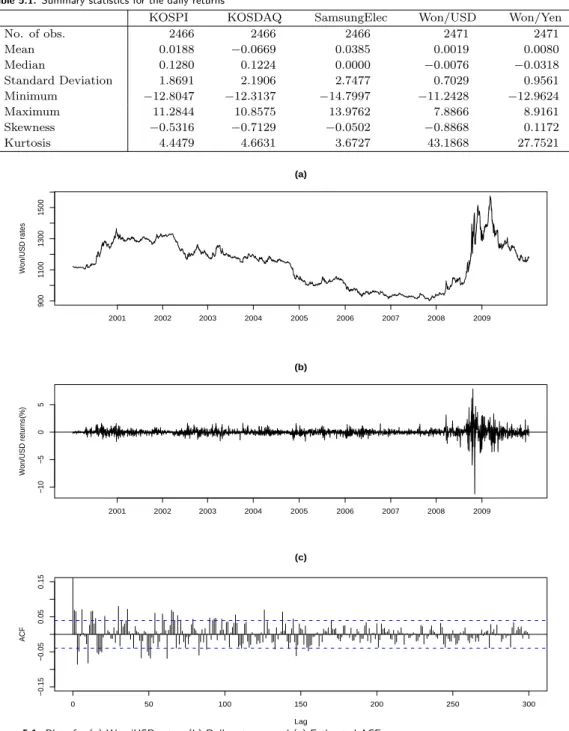
Table 5.1. Summary statistics for the daily returns

KOSPI KOSDAQ SamsungElec Won/USD Won/Yen

No. of obs. 2466 2466 2466 2471 2471

Mean 0.0188 −0.0669 0.0385 0.0019 0.0080

Median 0.1280 0.1224 0.0000 −0.0076 −0.0318

Standard Deviation 1.8691 2.1906 2.7477 0.7029 0.9561

Minimum −12.8047 −12.3137 −14.7997 −11.2428 −12.9624

Maximum 11.2844 10.8575 13.9762 7.8866 8.9161

Skewness −0.5316 −0.7129 −0.0502 −0.8868 0.1172

Kurtosis 4.4479 4.6631 3.6727 43.1868 27.7521

900110013001500

(a)

Won/USD rates

2001 2002 2003 2004 2005 2006 2007 2008 2009

−10−505

(b)

Won/USD returns(%)

2001 2002 2003 2004 2005 2006 2007 2008 2009

0 50 100 150 200 250 300

−0.15−0.050.050.15

Lag

ACF

(c)

Figure 5.1. Plots for (a) Won/USD rates, (b) Daily returns, and (c) Estimated ACF

is about 6 years from February 9, 2004 to the end of data for all series. In this period, there are

1466 (1471) trading days out of the whole 2466 (2471) days for the stock market data (the FX rates

data).

−15−10−50510

2005 2006 2007 2008 2009

99%

95%

Figure 5.2. Forecasted VaRs for KOSPI returns at confidence level 99% and 95% based on the QR method

Table 5.1 reports summary statistics for the daily returns of the whole period. It shows that the returns of FX rates are more leptokurtic than the returns of stock prices. Figure 5.1 depicts the movements of the Korean Won/USD rates and the daily return series, and its autocorrelation function(ACF). The ACF plot seems to suggest an existence of long range dependency, of which phenomenon is also true for Won/Yen rates, whereas this is not so significant for the three stock market returns. However, since autocorrelations are modest in size for all return series and various estimating periods, we only fit an AR(1) model to those series.

During the last 6 years of each series, we forecast daily VaRs at τ = (0.4%, 1%, 5%, 10%) based on the aforementioned three methods in Section 3 with the rolling scheme. Note that the VaR at τ = 0.4% indicates the value beneath which only one daily return possibly comes out within a year (about 250 trading days). In the rolling scheme, various estimation period lengths are utilized for each forecasting method, and subsequently, it is revealed that the performance varies in a large scale according to the estimation period length. On the basis of this result, we select T

= 1000 for both the QR and QML methods while in the historical simulation(HS) method, T

= 100 is selected for τ = (1%, 5%, 10%) and T

= 250 for τ = 0.4%.

Figures 5.2, 5.3 and 5.4 illustrate the daily VaR forecasting results for the KOSPI return series at

τ = 1% and 5% based on the QR, QML and HS methods, respectively. It can be readily checked

visually in Figure 5.4 that ignoring the conditional heteroscedasticity leads the VaR violations to

cluster and the HS VaRs to seriously underestimate losses in the periods when the volatility increases

(particularly when the global financial crisis hit the world in 2008). This poor performance is

measured by the backtesting and is reported in Table 5.2. In comparison to this, Figures 5.2 and 5.3

exhibit that the heteroscedasticity is well reflected in the QR and QML VaRs and the forecasting

is performed properly. The 95% and 99% QML VaRs in Figure 5.3 move in parallel since they are

based on the same estimates of GARCH parameters. In contrast the QR VaRs in Figure 5.2 do not

go in parallel exactly, since we obtain different estimates of GARCH parameters for each τ . This

feature often occurs even in simple linear regression models when we draw quartile lines conditional

on explanatory variables based on the least square or quantile regression fit.

−15−10−50510

2005 2006 2007 2008 2009

99%

95%

Figure 5.3. Forecasted VaRs for KOSPI returns at confidence level 99% and 95% based on the QML method

−15−10−50510

2005 2006 2007 2008 2009

99%

95%

Figure 5.4. Forecasted VaRs for KOSPI returns at confidence level 99% and 95% based on the HS method

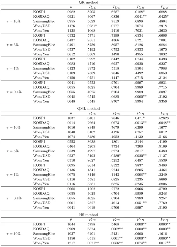
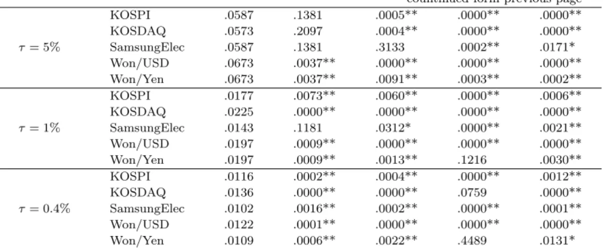
For the five return series, four confidence levels, and three different kinds of VaR forecasts, the

four backtesting methodologies described in Section 4 are implemented. Table 5.2 reports the

coverage rates ˆ p and p-values. With regard to the coverage rates, the number of acceptances from

the unconditional coverage tests at the 5% significance level is 19, 20 and 8 out of 20 tests in the

QR, QML and HS methods, respectively. This result indicates that the methods based on GARCH

models perform adequately and that the HS method does not perform inadequately according to

the criterion of the number of violations. However, the HS VaR forecasts turn out to perform poorly

in other backtesting results. Out of the 80 tests, the number of rejections is 5(2), 7(5) and 64(61) at

the 5%(1%) significance level in the QR, QML and HS forecasting strategy, respectively. Thus, it

Table 5.2. Coverage rates and p-values from backtesing for daily VaR forecasting QR method ˆ

p PU C PCC PLB PDQ

KOSPI .0982 .8205 .6287 .0188* .6888

KOSDAQ .0921 .3067 .0836 .0041** .0425*

τ = 10% SamsungElec .0955 .5629 .7519 .6898 .4804

Won/USD .1176 .0281* .0777 .7674 .2918

Won/Yen .1128 .1068 .2410 .7021 .2630

KOSPI .0532 .5771 .7399 .6534 .6606

KOSDAQ .0437 .2551 .4366 .5721 .7001

τ = 5% SamsungElec .0491 .8759 .8957 .8126 .9884

Won/USD .0537 .5192 .0752 .0533 .1670

Won/Yen .0612 .0569 .1490 .4955 .3032

KOSPI .0102 .9292 .8442 .0744 .6493

KOSDAQ .0082 .4710 .6927 .9920 .9227

τ = 1% SamsungElec .0123 .3972 .5518 .9504 .7988

Won/USD .0109 .7389 .7846 .4492 .8859

Won/Yen .0150 .0751 .1447 .0715 .3124

KOSPI .0041 .9553 .9701 .9997 .9931

KOSDAQ .0055 .4025 .6704 .9989 .7715

τ = 0.4% SamsungElec .0055 .4025 .6704 .9989 .8097

Won/USD .0048 .6545 .0685 .0000** .2192

Won/Yen .0048 .6545 .8707 .9994 .9356

QML method ˆ

p PU C PCC PLB PDQ

KOSPI .1037 .6401 .7846 .0471* .52828

KOSDAQ .0914 .2664 .0673 .0013** .0048**

τ = 10% SamsungElec .1016 .8349 .7679 .6299 .1677

Won/USD .1040 .6102 .4126 .6757 .8012

Won/Yen .1074 .3486 .4952 .4132 .5166

KOSPI .0553 .3638 .4801 .3144 .4199

KOSDAQ .0464 .5205 .7724 .7208 .9109

τ = 5% SamsungElec .0539 .4997 .5273 .3817 .6480

Won/USD .0537 .5192 .0289* .0020** .1127

Won/Yen .0510 .8627 .5252 .6487 .5539

KOSPI .0095 .8614 .8522 .9837 .9488

KOSDAQ .0136 .1841 .2244 .6805 .4464

τ = 1% SamsungElec .0075 .3149 .1143 .0008** .3249

Won/USD .0116 .5581 .6825 .5235 .8666

Won/Yen .0116 .5581 .6825 .5235 .8806

KOSPI .0068 .1202 .2772 .9966 .5799

KOSDAQ .0055 .4025 .6704 .9989 .9248

τ = 0.4% SamsungElec .0055 .4025 .6704 .9989 .9257

Won/USD .0061 .2327 .4613 .0051** .7769

Won/Yen .0041 .9619 .9706 .9997 .5190

HS method ˆ

p PU C PCC PLB PDQ

KOSPI .1044 .5798 .5468 .0000** .0000**

KOSDAQ .0969 .6874 .0002** .0000** .0000**

τ = 10% SamsungElec .1037 .6401 .5431 .0600 .1616

Won/USD .1156 .0515 .0001** .0000** .0000**

Won/Yen .1217 .0071** .0056** .0074** .0017**

countinued form previous page

KOSPI .0587 .1381 .0005** .0000** .0000**

KOSDAQ .0573 .2097 .0004** .0000** .0000**

τ = 5% SamsungElec .0587 .1381 .3133 .0002** .0171*

Won/USD .0673 .0037** .0000** .0000** .0000**

Won/Yen .0673 .0037** .0091** .0003** .0002**

KOSPI .0177 .0073** .0060** .0000** .0006**

KOSDAQ .0225 .0000** .0000** .0000** .0000**

τ = 1% SamsungElec .0143 .1181 .0312* .0000** .0021**

Won/USD .0197 .0009** .0000** .0000** .0000**

Won/Yen .0197 .0009** .0013** .1216 .0030**

KOSPI .0116 .0002** .0004** .0000** .0012**

KOSDAQ .0136 .0000** .0000** .0759 .0000**

τ = 0.4% SamsungElec .0102 .0016** .0002** .0000** .0001**

Won/USD .0122 .0001** .0000** .0000** .0000**

Won/Yen .0109 .0006** .0022** .4489 .0131*

NOTE: The symbol∗(∗∗) stands for rejection at the 5%(1%) significance level.

Table 5.3. Coverage rates and p-values from backtesting for simulated series—Sample 1

Model (a) Model (b)

ˆ

p PU C PCC PLB PDQ pˆ PU C PCC PLB PDQ

QR .0897 .1825 .2397 .8694 .5598 .0965 .6559 .4191 .0928 .5653 τ = 10% QML .0897 .1825 .2397 .8310 .5114 .0979 .7870 .3902 .2195 .5663 HS .1013 .8691 .8862 .9988 .0002** .1033 .6717 .4150 .6399 .0302*

QR .0455 .4266 .5556 .7794 .7523 .0551 .3802 .6253 .3040 .6711 τ = 5% QML .0469 .5825 .6080 .7782 .7976 .0551 .3802 .6253 .3002 .7816

HS .0544 .4465 .6961 .8584 .0007** .0612 .0569 .0127* .0148* .0011**

QR .0095 .8512 .8506 .0357* .2740 .0116 .5581 .3515 .1958 .0740 τ = 1% QML .0102 .9396 .8456 .0116* .4780 .0095 .8512 .2920 .2776 .1405

HS .0218 .0001** .0004** .6836 .0000** .0218 .0001** .0002** .4293 .0000**

QR .0054 .4074 .6754 .9989 .7449 .0041 .9619 .9706 .9997 .0240*

τ = 0.4% QML .0054 .4074 .6754 .9989 .7803 .0041 .9619 .9706 .9997 .1180 HS .0068 .1224 .2812 .9967 .3132 .0088 .0113* .0007** .0000** .0002**

NOTE: The symbol∗(∗∗) stands for rejection at the 5%(1%) significance level.

can be concluded that the QR and QML methods provide reasonable VaR forecasts for the return series. Further, by considering the overall testing results at the 1% significance level, it can be maintained that the QR method slightly outperforms and is more stable than the QML method.

Our findings strongly support that in GARCH models the proposed one-step-ahead VaR forecasting is the direct conditional quantile estimation method with a reasonable performance.

5.2. Simulation results

As seen in Figure 5.1, the daily returns of Won/USD and Won/Yen exchange rates exhibit a long range dependency. However, in the previous session we fitted an AR(1) model to specify the conditional mean since autocorrelation coefficients are moderate and the conditional mean has little impact on VaR forecasting. To justify this step, we implement the same VaR forecasting for simulated data following the FARIMA(1, d, 1)-GARCH(1, 1) model:

(1 − ϕB)(1 − B)

r

= (1 + θB)ε

,

Table 5.4. Number of rejections at the 5%(1%) significance level for all 10 samples

Model (a) Model (b)

PU C PCC PLB PDQ Total PU C PCC PLB PDQ Total QR 0 (0) 0 (0) 1 (0) 2 (1) 3 (1) 1 (0) 1 (0) 0 (0) 1 (0) 3 (0) τ = 10% QML 0 (0) 1 (0) 1 (0) 1 (1) 3 (1) 0 (0) 0 (0) 0 (0) 0 (0) 0 (0) HS 0 (0) 2 (2) 3 (1) 9 (8) 14 (11) 0 (0) 6 (3) 4 (3) 9 (7) 19 (13) QR 0 (0) 0 (0) 0 (0) 2 (1) 2 (1) 0 (0) 0 (0) 1 (0) 0 (0) 1 (0) τ = 5% QML 0 (0) 0 (0) 0 (0) 1 (0) 1 (0) 1 (0) 0 (0) 0 (0) 0 (0) 1 (0) HS 2 (1) 2 (1) 2 (1) 10 (9) 16 (12) 2 (0) 7 (3) 6 (3) 9 (9) 24 (15) QR 0 (0) 0 (0) 1 (0) 0 (0) 1 (0) 0 (0) 0 (0) 0 (0) 1 (0) 1 (0) τ = 1% QML 0 (0) 0 (0) 1 (0) 0 (0) 1 (0) 0 (0) 0 (0) 3 (0) 1 (0) 4 (0) HS 10 (9) 10 (9) 2 (0) 10 (10) 32 (28) 10 (10) 10 (10) 3 (2) 10 (10) 33 (32) QR 0 (0) 0 (0) 2 (2) 0 (0) 2 (2) 0 (0) 0 (0) 2 (2) 1 (0) 3 (2) τ = 0.4% QML 0 (0) 0 (0) 3 (3) 1 (0) 4 (3) 0 (0) 0 (0) 3 (3) 0 (0) 3 (3) HS 5 (3) 5 (2) 4 (2) 6 (5) 20 (12) 7 (2) 5 (2) 4 (3) 9 (5) 25 (12)

Table 5.5. Coverage rates and p-values from backtesting for 10-daily VaR forecasting

KOSPI Won/USD

ˆ

p PU C PCC PLB PDQ pˆ PU C PCC PLB PDQ

QR .0822 .4606 .1256 .0064** .0062** .0816 .4447 .2337 .2813 .4807 τ = 10% QML .0959 .8677 .3347 .0382* .0440* .0748 .2891 .2150 .2160 .2601 HS .1027 .9125 .0004** .0000** .0001** .1293 .2557 .1092 .0001** .2843 QR .0548 .7934 .6746 .6668 .3535 .0612 .5457 .4328 .7655 .7583 τ = 5% QML .0548 .7934 .6746 .6668 .2764 .0544 .8083 .5772 .1171 .3199 HS .0479 .9087 .5778 .6870 .5060 .0816 .1054 .2475 .0746 .1315 QR .0137 .6706 .8761 .9995 .6709 .0204 .2662 .4957 .9967 .8073 τ = 1% QML .0205 .2621 .4902 .9967 .5649 .0204 .2662 .4957 .9967 .7884

HS .0205 .2621 .4902 .9967 .3339 .0544 .0002** .0005** .0931 .0028**

NOTE: The symbol∗(∗∗) stands for rejection at 5%(1%) significance level.

ε

= √ h

η

,

h

= ω + αε

+ βh

,

where B is the backward-shift operator and η

are i.i.d. N (0, 1) random variables. We consider the following parameter values:

(a) d = 0.20, ϕ = 0.77, θ = 0.88, ω = 0.005, α = 0.15, β = 0.75, (b) d = 0.30, ϕ = 0.77, θ = 0.88, ω = 0.005, α = 0.15, β = 0.75,

where the parameters of FARIMA of Model (a) are fitted values of returns in Figure 5.1. Note that Model (b) has a larger memory parameter. We generate 10 samples of the same size as the returns of FX rates. Table 5.3 reports VaR forecasting results for the first samples of the two models. The number of rejections in 10 simulated samples are presented in Table 5.4. The result appears to be almost the same as in Section 5.1, which justifies the validity of our method.

5.3. 10-daily VaR forecasting

Although the result in Section 5.1 supports the validity of the proposed method when applied to

the daily VaR forecasting based on daily returns, practitioners also inquire to measure VaR for

multi-periods. However, since the conditional quantile function of multi-period returns in GARCH

models is not easily specified, our approach is not directly applicable to the multi-step-ahead VaR forecasting. In this subsection, we only implement 10-daily VaR forecasting based on 10-daily returns and examine its performance for the KOSPI and Won/USD data. Here we utilize the same period as in Section 5.1. The number of observations is 246(247) for KOSPI data (Won/USD data).

We select the estimation period length T

= 100 in implementing all the three methods. The results are reported in Table 5.5. Although the QR and QML methods perform well to a certain degree, it seems that the number of observations are not sufficient to make a solid conclusion about the (in)adequacy of these methods in contrast to what we have seen in Table 5.2, which actually supports the need to use the multi-step-ahead VaR forecasting. Considering its importance, we leave this as a task of our future study.

References

Berkowitz, J., Christoffersen, P. and Pelletier, D. (2009). Evaluating Value-at-Risk models with desk-level data, Management Science, published online before print.

Chernozhukov, V. and Umantsev, L. (2001). Conditional value-at-risk: Aspects of modeling and estimation, Empirical Economics, 26, 271–292.

Christoffersen, P. F. (1998). Evaluating interval forecasts, International Economic Review, 39, 841–861.

Engle, R. F. and Manganelli, S. (2004). CAViaR: Conditional autoregressive value at risk by regression quantiles, Journal of Business and Economic Statistics, 22, 367–381.

Francq, C. and Zako¨ıan, J. M. (2004). Maximum likelihood estimation of pure GARCH and ARMA-GARCH processes, Bernoulli, 10, 605–637.

Hartz, C., Mittnik, S. and Paolella, M. (2006). Accurate value-at-risk forecasting based on the normal- GARCH model, Computational Statistics and Data Analysis, 50, 3032–3052.

Hull, J. and White, A. (1998). Incorporating volatility updating into the historical simulation method for value at risk, Journal of Risk, 1, 5–19.

Kupiec, P. H. (1995). Techniques for verifying the accuracy of risk measurement models, Journal of Deriva- tives, 3, 73–84.

Lee, S. and Lee, T. (2010). Value at risk forecasting based on Gaussian mixture ARMA-GARCH model, Journal of Statistical Computation and Simulation, In press.

Lee, S. and Noh, J. (2009). Quantile regression estimator for GARCH models, Submitted.

W¨urtz, D., Chalabi, Y. and Luksan, L. (2002). Parameter estimation of ARMA models with GARCH/APA- RCH errors an R and SPlus software implementation, Unpublished manuscript.