Development of Hyperelastic Model for Butadiene Rubber Using a Neural Network

(1)

DOI: https://doi.org/10.7473/EC.2021.56.2.79

Development of Hyperelastic Model for Butadiene Rubber Using a Neural Network

Truong Thang Pham, Changsu Woo

^*

, Sanghyun Choi

^**

, Juwon Min

^**

, and Beomkeun Kim

^***,†

Department of Mechanical Engineering, Inje University, 197 Inje-ro, Gimhae-si, Gyeongnam 50834, Republic of Korea

*

Department of Nano Mechanics, Korea Institute of Machinery & Materials, 156 Gajeongbuk-ro, Yuseong-gu, Daejeon 34103, Republic of Korea

**

Daeheung R&T, 70-25, Seobu-ro 436 Beon-gil, Jillye-Myeon, Gimhae-si, Gyeongnam 50872, Republic of Korea

***

High Safety Vehicle Core Technology Research Center, Inje University, 197 Inje-ro, Gimhae-si, Gyeongnam 50834, Republic of Korea

(Received April 12, 2021, Revised April 26, 2021, Accepted May 4, 2021)

Abstract: A strain energy density function is used to characterize the hyperelasticity of rubber-like materials. Conventional

models, such as the Neo-Hookean, Mooney-Rivlin, and Ogden models, are widely used in automotive industries, in which the strain potential is derived from strain invariants or principal stretch ratios. A fitting procedure for experimental data is required to determine material constants for each model. However, due to the complexities of the mathematical expression, these models can only produce an accurate curve fitting in a specified strain range of the material. In this study, a hyper- elastic model for Neodymium Butadiene rubber is developed by using the Artificial Neural Network. Comparing the ana- lytical results to those obtained by conventional models revealed that the proposed model shows better agreement for both uniaxial and equibiaxial test data of the rubber.

Keywords: hyperelastic model, neural network, rubbers, stress/strain curves, Finite element analysis (FEA)

Introduction

Rubber-like and elastomeric materials are widely utilized for engineering applications such as rubber tires, engine mountings, seals, and shock absorbers and etc. The dominant property of these materials is their ability to elongate large deformation.

¹

A number of hyperelastic models are investigated to char- acterize the highly non-linear behavior of rubbers. Many attempts have been conducted to compare the results obtained from the constitutive models and experiments for the target materials.

^2,3

It shows that the conventional models have limits to match the data efficiently, i.e., they have difficulties capturing multi-axial deformation states of the hyperelastic materials.

Artificial neural network (ANN) with a capacity of capturing complex relationships between inputs and outputs has been used in many studies to construct mathematical models

between physical quantities. Using a neural network to model strain energy density function in terms of strain invariants, Shen et al. and Liang et al. developed hyperelastic models for incompressible rubber and elastomeric foams, respec- tively.

^4,5

Linka et al. introduced a general approach to con- stitutive artificial neural networks, which incorporates knowledge of rubber mechanics and experimental data to build a constitutive hyperelastic model.

⁶

Three aforementioned works also found a successful and efficient implementation of the models in commercial finite element software.

The target material of this study is Neodymium Butadiene rubber (NdBR), provided by Daeheung Rubber and Tech- nology. Its typical application includes tires (tread and side- wall), retreads, conveyor belts, and anti-vibration bushings.

This study represents a more efficient model for hyperelastic materials, which helps engineers to obtain better design and analysis of mechanical parts made of NdBR.

†Corresponding author E-mail: [email protected]

(2)

Experimental

1. Continuum mechanics of rubber

In the following, the mechanics of rubber material are briefly revised. The local gradient of deformation is denoted . The right Cauchy-Green deformation tensor is then related to by:

(1) The strain invariants, denoted I

1

, I

2

, I

3

, are given by:

(2)

Hyperelastic materials normally experience large deforma- tion in many applications. Due to large strain problems, two major stress tensors are considered and defined, the true stress tensor s and the first Piola-Kirchoff (also called the nominal) stress tensor . These physical quantities are related by:

(3) In this study, our investigated material is assumed to be homogeneous, isotropic, rate-independent, and incompress- ible. Therefore, the kinematic condition must be satisfied, which is represented by: . The first Piola- Kirchoff stress tensor can be rewritten:

(4)

where  is the Lagrange multiplier associated with the

incompressibility constraint.

For further details, readers are encouraged to refer for example to.

⁷

2. Conventional Hyperelastic models

In this section, we shortly discuss the formulations of widely used hyperelastic models for rubber-like materials.

Neo-Hookean model is one of the simple models for incompressible materials where the strain density function is a linear function of only the first strain invariant as follows:

(5) A Mooney-Rivlin model is introduced by Melvin Mooney and Ronald Rivlin, where the strain energy density function is a linear combination of two strain invariants:

⁸

(6) An Ogden model is a different approach to those two above models.

⁹

This model expresses the strain energy density function in terms of principal stretch ratios. For example, the third- order Ogden model has that function defined by:

(7)

3. Neural network-based modeling of rubber

In this study, the neural network-based hyperelastic model is investigated to reproduce theoretically the stress-strain curves obtained from uniaxial and equibiaxial tension of industrial rubber used in automotive engine bush. The input F

F C F F 

T

1

2 2

3

( )

1 ( ) ( )

det( ) 2 I tr C

I tr C tr C

I C



 

   



P

det( )

^T

P  F F 

^

det( )

3

1 J  F   I



¹



1 2

T

2

T

W W W

P F F I F FC F

F 

^

 I I  

^

  

            

10

(

1

3) W C I  

10

(

1

3)

01

(

2

3)

W C I    C I 



¹ ² ³



1

3

N n

n n

n n n

W    

^ ^ ^



 



  

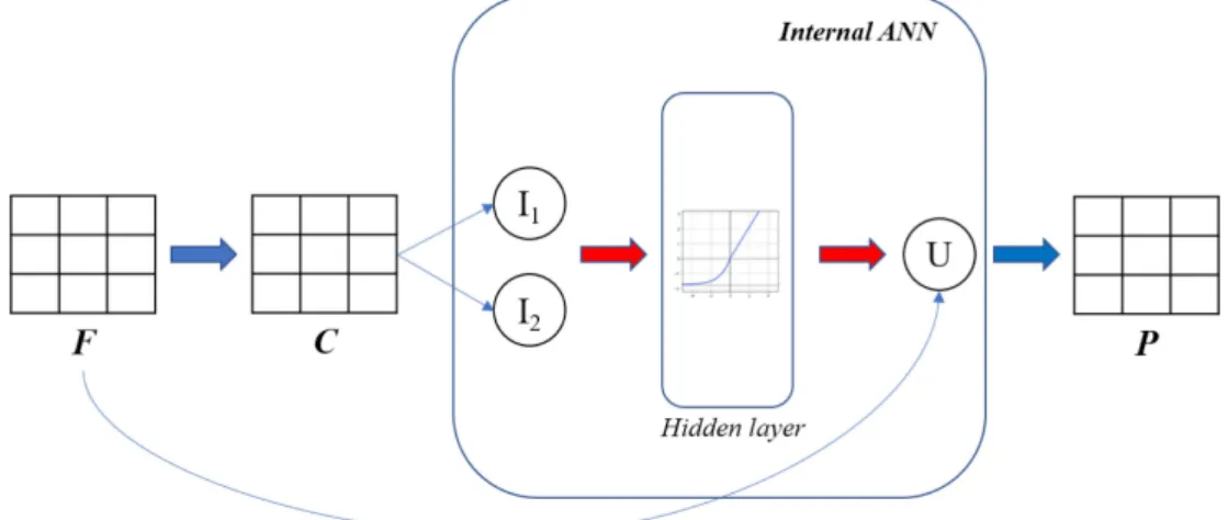
Figure 1. Structure of the neural network (red arrow denotes trainable weights between two dense layers).

(3)

of this model is deformation gradient (in the shape of 3×3), and the output is nominal stress tensor (also in the shape of 3×3). The structure of the model is demonstrated in Figure 1.

Conventional models for incompressible rubber-like mate- rials such as Ogden, Neo-Hookean, Mooney-Rivlin, define strain energy density (denoted U) explicitly as an expression of stretch ratios or strain invariants. In the proposed method of this study, this relationship is undecided and left open to learning from data using an internal ANN with one hidden layer and a Scaled Exponential Linear Unit (SELU) activa- tion function.

¹⁰

This internal ANN accepts two strain invariants as input and results in a scalar value of strain density potential, as shown in Figure 1.

The hyperparameters in the model include the number of hidden units, learning rate, the initialization methods, the number of epochs, and batch size.

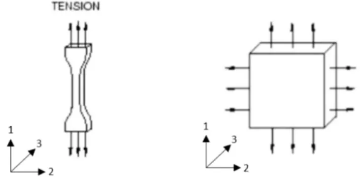
4. Material testing method

Two testing modes are conducted to obtain stress and strain data, as demonstrated in Figure 2 with a fixed coordinate sys- tem. These experimental data are then processed into the inputs and outputs of the model. The details are discussed in the next section. It is important to note that the rubber spec- imen should be stabilized by stretching several times to reach two or three maximum strain levels beforehand.

¹¹

4.1. Uniaxial tension test

This test creates a deformation state where there is no lat- eral constraint to thinning dimension. Normally, the length of the specimen has to be at least 10 times higher than the width and thickness. The deformation gradient and the engi- neering stress tensor is expressed below:

, (8)

where l is the primary stretch ratio, P is the load, and A

0

is the initial cross-section area of the specimen.

4.2. Equibiaxial extension test

A state of equal strain in two directions is created in this test. The equal biaxial strain state may be achieved by radi- ally stretching a circular disc. The deformation gradient and the engineering stress tensor at the center of the disc are defined by:

(9)

A

0

is the original area normal to the width and the height of the specimen. A straight line of initial length L

0

is marked in the specimen and then measured the deformed length, L, using a laser extensometer. The primary stretch ratio, l, is cal- culated by: . The equibiaxial stress, s, is defined by:

, where P is the sum of the forces normal to the width and the height.

5. Training progress and implementation into ABAQUS

The model is implemented in the Python-based machine learning library Keras-Tensorflow, using symbol-to-symbol automatic differentiation in the library.

¹²

The raw data from experiments are processed to get the stable stress-strain curves in uniaxial and biaxial modes.

Thus, the test set of deformation gradient inputs and engi- neering stress tensor outputs is obtained. Afterward, they are applied to the training process. The number of hidden units in the hidden layer is varied to have reasonable curve fitting F

P

F P

0.5 0.5

0 0

uniaxial

F





 

 

  

 

 

/

0

0 0

0 0 0

uniaxial

P A

P



 

 

 

F P

2

0 0 0 0

0 0 , 0 0

0 0 0 0 0

equibiaxial equibiaxial

F P

 



^



   

   

    

   

   

0

L

 L

0

P

 A

Figure 2.

Illustration of testing methods.

Table 1.

Hyperparameters of the Neural Network

Parameters Value/Specification

Learning rate 0.005

Optimization method Adams (default 1, 2, ε) Initialization method Glorot Uniform

Epochs 3500-4000

Batch size 8

Loss Mean absolute percentage error

Hidden units 7 (6-8)

(4)

compared to experiments, depending on the complexity of the multi-axial stress-strain relationship of the material. In this rubber material, we found that 6-8 units in the hidden layers result in a satisfactory fitting. The training algorithm is Adam with default parameters. The hyperparameters of the model are shown in Table 1.

In this work, we compared the neural network-based model with three widely used conventional hyperelastic models:

Ogden 3

^rd

, Neo-Hookean, Mooney-Rivlin. The material con- stants for these models are obtained from ABAQUS.

Results and Discussion

The stress level from both the constitutive model by neural network and conventional models are extracted for compar- ison.

1. Equibiaxial test results

Figure 3 shows the results of hyperelastic models for the uniaxial tension test. As shown in Figure 3, the neural net- work model has better agreement with experiments than the

Figure 3. Equibiaxial extension test results.

Figure 4. Uniaxial tension test results.

(5)

conventional models do. Ogden 3

^rd

model fits accurately up to a strain level of about 20%. In addition, Mooney-Rivlin and Neo-Hookean models match the data in a strain range of 30%-60%.

2. Uniaxial test results

The results for the uniaxial test are shown in Figure 4. The neural network model fits the experiments efficiently. For a low strain range below 40%, conventional models are not enough to represent the non-linearity of the material. Ogden 3

^rd

model and Mooney-Rivlin model match the data in a moderate strain range of 45%-65%.

3. Implementation in ABAQUS

To verify the implementation of the proposed hyperelastic model using a neural network in a commercial FEA software, the UHYPER subroutine of ABAQUS was coded based on the fully trained model. The analysis of the biaxial extension test is reproduced, and Figure 5 shows the strain distribution.

Conclusions

In this study, a hyperelastic model for rubber material using a neural network was developed and implemented suc- cessfully into FEA software. A combination of test data from uniaxial and equibiaxial experiments was used to train the model. A good agreement between experiments and the pro- posed model is achieved. In comparison with widely used conventional models, the neural network-based shows more

efficient curve fitting results. Effects due to more training data from different test modes such as torsion, pure shear or simple shear and the structure of the neural network should be investigated for future study.

Acknowledgements

This work was supported by the Regional Innovation Proj- ect based on local Government-University Cooperation [Smart ManufacturingEngineering for Innovation Platform in Gyeongsangnam-do] grant funded by the Ministry of Edu- cation [National Research Foundation of Korea (NRF)].

References

1. Werner Hoffman, “Rubber Technology Handbook”, Hanser, (1989).

2. B. Kim, S. B. Lee, J. Lee, S. Cho, H. Park, S. Yeom, and S. H.

Park, “A comparison among Neo-Hookean model, Mooney- Rivlin model, and Ogden model for Chloroprene rubber”, Int.

J. Precis. Eng. Manuf., 13, 759 (2012).

3. G. Marckmann and E. Verron, “Comparison of hyperelastic models for rubber-like materials”, Rubber Chem. Technol., 79, 835 (2006).

4. Y. Shen, K. Chandrashekhara, W. F. Breig, and L. R. Oliver,

“Neural network based constitutive model for rubber mate- rial”, Rubber Chem. Technol., 77, 257 (2004).

5. G. Liang and K. Chandrashekhara, “Neural network based constitutive model for elastomeric foams”, Eng. Struct., 30, 2002 (2008).

6. K. Linka, M. Hillgärtner, K. P. Abdolazizi, R. C. Aydin, M.

Itskov, and C. J. Cyron, “Constitutive artificial neural net-

Figure 5. Analysis results of equibiaxial tension test. (a) Undeformed body, (b) Strain distribution of deformed body

(6)