Railway Track Maintenance Scheduling using Artificial Bee Colony and Harmony Search

http://dx.doi.org/10.5369/JSST.2016.25.2.91 pISSN 1225-5475/eISSN 2093-7563

Railway Track Maintenance Scheduling using Artificial Bee Colony and Harmony Search

Ki-Dong Kim ¹ , Sung-Soo Kim ^1,+ , Duk-Hee Nam ² , and Hanil Jeong ³

Abstract

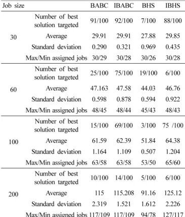
The objective of this paper is to propose a heuristic algorithm to optimize the railway track maintenance scheduling, a NP-hard prob- lem, by reflecting conditions of the actual field more quickly and easily. We develop the mechanism based on Binary Artificial Bee Col- ony (BABC) and Binary Harmony Search (BHS), and verify their performance through simulation experiments. Our proposed BABC and BHS mechanisms were applied to problems composed of 30, 60, 100, and 200 operations for railway track maintenance scheduling to carry out experiments and analysis. On comparing it with the results solved by CPLEX, it is found that the mechanism could present an optimal solution within limited time by user.

Keywords: Railway Track Maintenance Scheduling, Artificial Bee Colony, Harmony Search

1. Background and Purpose of the Study

The most efficient and effective maintenance schedule is established by considering the abilities and availabilities of various resources such as manpower and equipment in the track maintenance field [15]. An efficient and effective maintenance plan can be explained in various ways. The criterion would be varied depending on the purpose or circumstances of the organization carrying out the maintenance. However, performing more jobs with given resources for an appropriate period is the most general and common purpose for optimization of a maintenance schedule.

At present, maintenance jobs for railway tracks are carried out through various methods depending on the conditions of the field.

Therefore, field conditions reflected in a schedule also show a variety of differences. This paper proposes a methodology applying a heuristic algorithm for flexible handling of such a

situation and a quicker establishment of a schedule.

Even though a heuristic algorithm could not guarantee optimal solutions, it can present optimal or best solutions within a short time or period given by schedulers. Furthermore, it also has an advantage that it can solve various problems more easily.

Therefore, various conditions at the railway track maintenance fields can also be reflected more easily to optimize it.

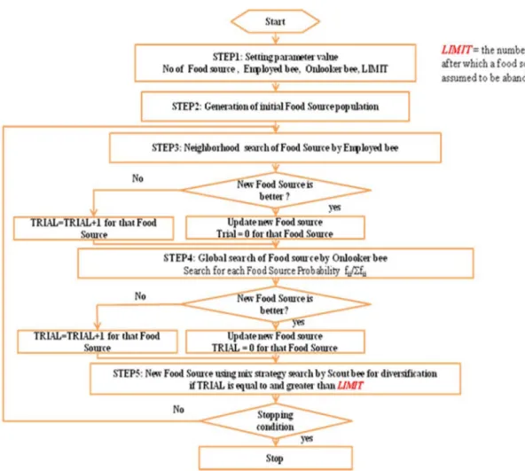
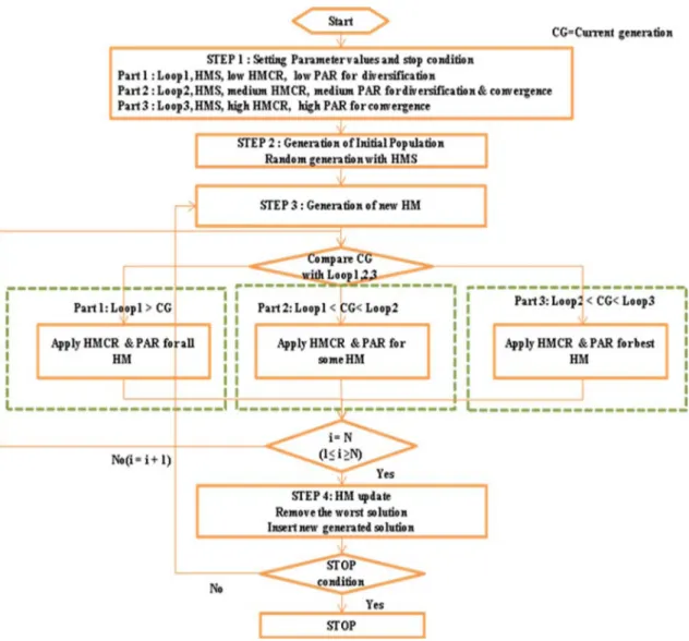
Among them, Artificial Bee Colony (ABC) and Harmony Search (HS) have been actively studied, their performances were proved, and related studies are constantly being carried out even in resource assignment and scheduling fields[2,6,7].

The purpose of this paper is to mathematically model the railway track maintenance scheduling problem and propose a mechanism that can be applied to obtain the best solution to the track maintenance schedule with sample data of KORAIL’s maintenance history of high-speed railway tracks.

2. Status of Related Studies

Present methods which are used to solve a resource assignment or scheduling problem in various fields could also be exploited as a method to solve optimization problems for track maintenance scheduling. As there is an availability of several resources, which are able to carry out a single job process in the problem for track maintenance scheduling covered in this paper, it develops a correlation with a parallel machine scheduling problem[3]. The parallel machine scheduling problem with non-preemptive jobs for minimizing completion time is known as NP-hard[1], which corresponds with the scheduling problem to solve in this paper.

*This study was supported by 2013 Research Grant from Kangwon National University

1

Department of System & Management Engineering, College of Engineering, Kangwon National University, Republic of Korea

2

M&S TFT, Huneed Technologies, Republic of Korea

3

Department of Computer Engineering, College of Engineering, Daejeon University, Republic of Korea

+

Corresponding author: [email protected] (Received: Mar. 17, 2016, Accepted: Mar. 29, 2016)

This is an Open Access article distributed under the terms of the Creative Commons Attribution Non-Commercial License(http://creativecommons.org/

licenses/bync/3.0) which permits unrestricted non-commercial use, distribution,

and reproduction in any medium, provided the original work is properly cited.

The parallel machine scheduling problem has been actively studied since the 1960s. Li[9] reviewed models for problems to minimize total weighted completion time of asymmetric parallel machines, and McNaughton[10] developed an algorithm to minimize the maximum task completion time (make span) in symmetric parallel machines.

With regard to track maintenance scheduling problems, Oh[14]

suggested a model loadable to commercial software for long-term scheduling of ballast tamping jobs, and Masashi MIWA[11]

presented a model to solve scheduling problems for ballast tamping jobs of MTT (Multiple Tie Tamper) in terms of minimizing maintenance cost.

In actual track maintenance fields, however, there are many on- site conditions to be considered as constraints, and it is quite difficult to simplify and adjust them to existing defined problems.

In addition, since all the on-site conditions are different depending on types or properties of the site, there are differences for constraints which are to be applied. This paper defines constraints to be reflected in common at each site through on-site investigation and analysis on related data. It can be referred as the foundation for scheduling which is suitable to each site’s conditions, and a methodology applying defined constraints may also be the basis to apply constraints arisen according to the on- site conditions.

3. Problems of Railway Track Maintenance Scheduling

This section gives a brief introduction to railway maintenances and a mathematical model of railway track maintenance scheduling problem.

In this paper, a job is referred to as a track maintenance job.

Each job has its own properties such as job type, due date, working section, and processing time. The type of job is determined depending on the kinds of abnormal conditions of railway tracks of that section. There are many types of jobs such as manual tamping, mechanical tamping (spot, overall tamping, etc.), gravel arrangement, resetting poles, and rail support welding etc. Manual and mechanical tamping occupies most of the workloads in actual. There are various types of resources available for each type of job. A job of manual tamping is generally carried out by manpower. Mechanical tamping can be divided into spot tamping and overall tamping, but there is no definite criteria on which these two types can be classified. In the field, however, overall tamping is generally carried out for overall ballast tamping

where the section of the job is relatively long, and spot tamping is carried out where the section is short and partial ballast tamping is required[17].

Overall tamping is usually carried out through an MTT. The MTT is an equipment for ballast tamping, which is mostly used in a job which involves correcting wrong tracks on gravel. The MTT usually performs horizontal tamping jobs by moving its tamping bar up and down through fluid pressures. Spot tamping is usually carried out through an STT (Switch Tie Tamper). The STT is an equipment to originally harden the branch area which is among the three main weak spots (curve area, joint area, and branch area) of tracks. Since it can also be worked in regular sections as well as the branch areas, it has been widely used in the entire sections[16].

Even though the resources available for a job are generally defined on the basis of each type of a job in the track maintenance field, it may be differently set according to the working environment or worker’s experiences. For example, although spot tamping is generally carried out by STT equipment, it could also be carried out by manpower according to the scheduler’s intention. The scheduler decides the type of job according to the kind of maintenance required and available resources. As a consequence, each job has its type and available types of resources having different capacities for each job type[17,18].

Due date of a job is the last day when the job has been carried out. A working section of a job is the geographical interval on which the maintenance is needed. A working section has its starting and ending points. The distance from a starting point to an ending point is called an extension, which determines the processing time of a job. Thus, the processing time of a job is dependent on the extension, type of a job, and used resource type.

There is only one interval per day which lasts for four hours, during which the train is not running. Maintenances are performed at this time. Usually the jobs are assigned a resource which is relatively close. The resource needs setup time for a day’s jobs which includes moving time to the place and preparing and arranging time for equipment.

A mathematical model is suggested for the track maintenance scheduling problem as follows. Indexes, parameters, and decision variables used in the model are described in the beginning.

●

Indexes and parameters = job number ( )

= time period number ( , unit: day) = resource number ( )

= starting point of the working section of job j

j 1 j J ≤ ≤

t 1 t T ≤ ≤

r 1 r R ≤ ≤

F _j

= ending point of the working section of job j = due date of job j

= processing time of job j by resource r (unit: minute) = set of available resources for the job j

= set of jobs that could be processed by resource r = capacity(total available time) of resource r at period t (unit: minute)

= setup time for human resources = setup time for mechanical resources

= set of mechanical resources = set of human resources

= maximum movable distance of resource r, corresponding only to human resources

=Big number M

●

Decision variables

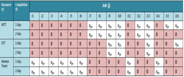
= 1 if the job j is processed by the resource r during the period t, otherwise 0

= the largest ending point of jobs to be assigned to the resource r during the period t

= the smallest starting point of jobs to be assigned to the resource r during the period t

●

0-1 integer programming for track maintenance Scheduling (1)

Subject to

≤ 1, ∀j (2)

≤ 1, ∀j (3)

= 0, _∀j (4)

≤ 1, ∀j (5)

= 0, ∀j (6)

∀t (7)

∀t (8)

, _∀ j, _∀ t, _∀ r (9)

, _∀ j, _∀ t, _∀ r (10)

∀ r, _∀ t (11)

Sections which miss the working opportunity would incur greater additional expenses due to the progress of abnormal states.

Furthermore, expenses would be incurred for additional manpower or equipment if a job could not be processed within its due date[12]. The objective function for problems to optimize the track maintenance schedule to carry out as many jobs as possible within its due date is given in equation (1).

By equation (2) each job should be assigned for only a day and only by a resource. Equations (3) and (4) describes that each job should be assigned to the resources that could process the job.

Equations (5) and (6) mean that a job should not be done on any day over its due date.

Equations (7) and (8) are for time capacity of resource r. Since can have a negative value for days when resources are not available, possible errors due to negative values are prevented by taking max for it as zero. Equations (9) and (10) are for calculating the maximum and minimum distances of jobs assigned from each resource. By equation (11) all the jobs which are assigned to a human resource are within the maximum movable distance of that resource.

4. Mechanism to Solve the Railway Track Maintenance Scheduling Problem

4.1 Description of BABC and IBABC Mechanism The ABC algorithm was introduced by Karaboga in 2005 for the first time. It is an algorithm made from motivation by intelligent behaviors of honeybees finding food by themselves[4].

The mechanism of Binary Artificial Bee Colony (BABC) based on the ABC algorithm can be explained as follows: steps of setting parameters, generating initial solutions, searching solutions by employed bees, searching solutions by onlooker bees, and searching solutions by scout bees according to the study by Karaboga et al.[4].

In the study by Karaboga et al.[4], there is a problem that a new solution arbitrarily generated by scout bees in the step searching solutions by them has poorer quality compared to existing solution T _j

D _j P _rj SR _j SJR _r C _rt

RA _h RA _m SMR _m SHR _h LT _r

BigM

x _jtr

ld _rt

sd _rt

Maximize x _jtr

r 1 = R

∑

t 1 = T

∑

j 1 = J

∑

x _jtr

r 1 = R

∑

t 1 = T

∑

x _jtr

r SR ∈

∑

t 1 = T

∑

x _jtr

r SR ∉

∑

t 1 = T

∑

x _jtr

r 1 = R

∑

t D ≤

∑

x _jtr

r 1 = R

∑

t D >

∑

P _jr • x _jtr ≤ max C ( _rt – RA _h , 0 ) r SHR , ∈ h ,

j SJRr ∈ ∑

P _jr • x _jtr ≤ max C ( _rt – RA _m , 0 ) r SHR , ∈ _m ,

j SJRr ∈ ∑ T _j • x _jtr ≤ id _rt

F _j + BigM • ( 1 x – _jtr ) sd ≥ _rt ld _rt – sd _rt ≤ LT _r

C _rt – RA _h

groups which are repeatedly improved. Even though generation of arbitrary solutions can give a wide range of solutions, overall performance of searching an optimal solution could be decreased as the number of these solutions increase. This paper proposes the following Improve Binary Artificial Bee Colony (IBABC) method to generate a new solution such that the quality of solutions is not significantly different compared with the existing solutions, besides the randomly searched solutions through scout bees. The IBABC has the same steps as the BABC except for the step 5. The step 5 combines solutions of the existing food source to generate a new solution. Each decision variable of solutions to be newly generated, select one of the existing food sources with the probability of the following equation (12) and the corresponding decision variable’s value of selected food source is applied. Scout bees determine every decision variable’s value of a new solution in this way.

(12)

Where i = indexes of each food source ( ), = probability that the i th food source is selected among all the food source,

= evaluated value of the i th food source The flow chart of IBABC is as Fig. 1.

4.2 Description of BHS and IBHS Mechanism The Harmony Search (HS) is an algorithm developed by introducing a musical concept of creating a perfect harmony, which was developed on the basis of performing processes of jazz musicians finding better conditions of harmony[2]. The harmony memory considering rate (HMCR) and pitch adjust rate (PAR) of BHS algorithm are quite important parameters in determining the performance of the algorithm. If the HMCR is large, it is difficult to get out of solution’s range given by the existing harmony memory (HM), as a result, the searching area for solutions becomes narrower. It means that solutions could be more intensively searched. On the contrary, if the HMCR is small, the number of p _i 1 1 e ⁄ ( + ^{– v}

) v _i fit _i fit _n , ( – 4 v ≤ ≤ _i 4 )

n 1 = SN

⁄ ∑

⎝ = ⎠

⎜ ⎟

⎛ ⎞

,

=

1 i SN ≤ ≤ p _i

fit _i

Fig. 1. Flow Chart of IBABC

decision variables arbitrarily generated is increased and thus, the searching area becomes wider. The pitch adjusts a solution’s value within a fixed range. If the PAR becomes larger, the probability to carry out the pitch adjustment also becomes higher such that the searching area for solutions becomes wider and if it becomes smaller, the searching area for solutions also becomes narrower.

The Improve Binary Harmony Search (IBHS) follows the method as shown in the flow chart in Fig. 2. The number of generations from step 1 to the time satisfying the stop condition is divided into total three parts of early, mid, and late phases. The HMCR and PAR are respectively set to be applied to each part. To widen early solution’s area for searching solutions, the HMCR is set as the smallest of the three parts, and the PAR as the largest. The mid search phase for solutions sets the HMCR as the second smallest, and the PAR as the second largest. The late search phase for solutions sets the HMCR as the largest, and the PAR as the smallest. The step 2 and 4 are identical to the BHS. The step 3 applies parameters to each part

suitable to the number of each generation. At this time, the part 1 generates new solutions for every HM, however, the part 2 generates new solutions only for some HMs with a good evaluation value among all HMs. The part 3 is targeted only at a HM with the best evaluation value among all HMs.

4.3 Application of IBABC and IBHS to the Railway Track Maintenance Scheduling Problem

This section solved a simple problem for track maintenance scheduling with the IBABC and IBHS mechanisms. The used data is referring to the KORAIL’s maintenance history data for high-speed railway tracks.

4.3.1 An Example for the Railway Track Maintenance Scheduling Problem[12]

Table 1 shows data arranging information for the example.

Fig. 2. Flow Chart of IBHS

Firstly, the schedule establishment period is set as two days of March from first to second. The available resources are mechanical resources, which are targeted at a MTT, a STT, and a manpower team. The maximum working time available in a day for the manpower team is 180 minutes including the free time between working, and for the MTT and STT is 120 minutes. The maximum working distance available for the manpower team is assumed as 2000m. The type of jobs that each resource carries out are such that the MTT carries out the job types 1 and 2 , the STT does the job type 2, and the manpower team does the job type 3.

4.3.2 Satisfying constraints of the heuristic algorithm For solving the problem, this paper expressed solutions to contain two meanings of available days for each job and resources for each job. Such an expression for solutions is used in both the IBABC and the IBHS. The in Fig. 2 below would have a value of 1 if the job j is carried out with the resource r during the period t, otherwise it would have a value of 0. The following Fig.

3[12] shows the representation method of solutions for example data in Table 1.

Areas possible and impossible to represent solutions could be x _jtr

Table 1. Example Data[12]

Job number Job type Starting point (m)

Termination point (m)

Section length (m)

Working time (min)

Required completion days (due date)

J1 3 10 13 3 30 2

J2 3 5 9 4 40 2

J3 3 1,927 1,930 3 30 2

J4 3 422 432 10 80 2

J5 3 2,500 2,575 25 100 2

J6 3 617 620 3 30 2

J7 1 3,000 3,080 80 60 2

J8 1 105 135 30 30 2

J9 2 990 1,000 10 10 2

J10 2 305 310 5 5 2

J11 3 3,044 3,053 9 90 2

J12 1 200 219 19 20 2

J13 2 3,077 3,097 20 40 2

J14 3 2,233 2,243 10 30 2

J15 1 3,120 3,125 5 50 1

J16 2 1,997 2,020 23 100 1

Fig. 3. Representation of Solution [12]

set through the above technique. The area impossible to express solutions represents the days outside the range of demand date for completion given for each job and the areas that assigns a value of 0 other than the decision variable in advance into resource areas makes it impossible to carry out the corresponding job as shown in Fig. 4[12]. Equations (2), (3), (4), (5), and (6) could be satisfied through it. Areas possible and impossible to represent solutions could be set through the above technique. The area impossible to express solutions represents the days outside the range of demand date for completion given for each job and the areas that assigns a value of 0 other than the decision variable in advance into resource areas makes it impossible to carry out the corresponding job as shown in Fig. 4[12]. Equations (2), (3), (4), (5), and (6) could be satisfied through it.

The IBABC and IBHS can make initial solutions or neighboring solutions (new solution for the IBHS.) It could not be assumed that solutions made after searching the neighborhood of early solutions would satisfy the equations (7), (8), and (9.) But it could be said that the solutions not satisfying equations (7), (8),

and (9) are infeasible solutions, a procedure is surely needed to make these infeasible solutions into feasible ones.

In the track maintenance scheduling problem, solutions available through a pure solution search of the heuristic algorithm include so many infeasible solutions. Furthermore, it would search more infeasible solutions to maximize the assigned amount of job.

Therefore, infeasible solutions made after searching the neighborhood of early solutions would be changed into feasible solutions through the following feasible solution search procedure.

The feasible solution search procedure to satisfy the constraint equation (7) is as follows.

Step 1: For resource r, find and among jobs assigned in day t, loop = 0

Step 2: Find value, if it is larger than , add 1 into the loop then go to step 3, otherwise go to step 4

Step 3: If the loop is odd, assign 0 into the job value assigned to , and if the loop is even, assign 0 into the job value assigned to , then go to step 1

Step 4: If t = T, go to step 5, otherwise go to step 1, then t = t+1 x _jtr

x _jtr

ld _rt sd _rt

ld _rt – sd _rt LT _r

x _jtr

ld _rt x _jtr

sd _rt Fig. 4. Representation of Zero area [12]

Table 2. Optimal job assignment for 16 job sizes

Job size Mechanism Resource of assigned job Day of assigned job Number of job assignment

1 2

16

IBABC

Human Team J1,J2,J4,J6 J3,J5,J14 7

MTT J7,J9,J15 J8,J10,J12,J13 7

STT J16 - 1

Number of job assignment 8 7 15

IBHS

Human Team J3,J11,J14 J1,J2,J4,J6 7

MTT J8,J15 J7,J12 4

STT J10,J16 J9,J13 4

Number of job assignment 7 8 15

Step 5: If r = R, stop, otherwise go to step 1, then r = r+1, t = 1

The feasible solution search procedure to satisfy the constraint equations (8) and (9) is as follows.

Step 1: For resource r, find the sum P _rj of working time of every job assigned in day t

Step 2: After finding the maximum daily available time of the resource r (if manpower, , or if equipments ) compare it with the sum of P _rj of every job assigned to resource r in day t, and if P _rj is larger, go to step 3, otherwise go to step 4.

Step 3: After assigning 0 into value of the job j with largest working time among all jobs j assigned for resource r in day t, go to step 1

Step 4: If t = T, go to step 5, otherwise go to step 1, then t = t+1 Step 5: If r = R, stop, otherwise go to step 1, then r = r+1, t = 1 4.3.3 Results of solving the example

As a result of solving the example, it can be confirmed that the result of both the methods IBABC and IBHS assigned 15 jobs of total 16 jobs. The result assigning 15 jobs of 16 ones is a result which satisfies the objective function as much as possible and it is confirmed by solving the problem with the CPLEX. Table 2 below shows the result assigned in the example, and Fig. 5 represents the solution search procedure.

With the result of job assignment, it is confirmed that all the constraints are satisfied through the feasible solution search procedure in section 2.3.2. For example, from solutions with the

IBABC, jobs assigned to the human team in the first day are J1, J2, J4, and J6, which are of job type 3. It can be found that total working time (30 + 40 + 80 + 30) for assigned jobs does not exceed 180 minutes, and total working distance is also 615m (620 – 5,) which does not exceed 2,000m. It can be confirmed from jobs assigned to every resource in the first and second days, and checked that all constraints are satisfied.

5. Experiments and Analysis Results

The track maintenance scheduling problem, which applies the heuristic algorithm proposed in this paper, was programmed with C++ of Microsoft’s Visual Studio 2005 and the experiment was conducted on a notebook computer of Intel(R) Core(TM) 2 Duo with CPU P 8600 @ 2.40 GHz and RAM 2.0 GB specifications.

Furthermore, to evaluate the performance and efficiency of the method solving the track maintenance scheduling problem applying the heuristic algorithm, it was compared with solutions of the numerical model with the CPLEX of ILOG product group.

The CPLEX could present an optimal solution with the numerical model.

Experiments were targeted at the job size of 30, 60, 100, and 200 during 7 days of schedule establishment period. Three types of jobs and three resources were used for the job size of 30, 60, and 100 and four resources were used for the job size of 200 for increasing the assignment rate. The type of job used was one of the following: manual tamping which is worked by human teams, C _rt – RA _h C _rt – RA _m

x _jtr

Fig. 5. Trend of convergence for 16 jobs

the mechanical tamping (overall tamping) by the MTT, and the mechanical tamping (spot) by the STT. For the job size of 30, 60, and 100, schedules for a resource were established by a human team, a MTT, and a STT respectively, and for the job size of 200, schedules were established by two human teams, a MTT, and a STT. Among the capacities of resources, actual available working time except the free time was 120 minutes at the maximum for mechanical jobs, and 180 minutes for manual jobs. For manual jobs, the maximum movable distance for a day was set as 2,000m.

Input data was made based on the form of track maintenance history data for high-speed railways[17, 18].

Tables 3 and 4 show optimal parameters found through simulations. Table 3 represents optimal parameters used in the BABC and the IBABC, and Table 4 represents optimal parameters used in the BHS and the IBHS. Subsequently, every experiment was conducted applying the optimal parameters.

5.1 Comparison between Conventional and Improved Mechanisms

To compare the improved mechanisms with the existing mechanisms, experiments were conducted for methods of BABC, IBABC, BHS, and IBHS in which each method was carried out 100 times for each job size. In addition, the average assigned amount of job, standard deviations, and the maximum and minimum assigned amount for each experiment was compared.

As a result of experiments, the difference was clearly showed for the BHS and the IBHS, and the latter solved better results for

the maximum value as well as the average value. Although the BABC solved better results than the BHS on the average, the IBHS could solve better results than the IBABC as well as the BABC. However, it confirms that the existing mechanism generally solved more stable results for standard deviations. In particular, standard deviations of BHS and IBHS showed relatively large differences. The following Table 5 shows the results of experiments.

The following Fig. 6 shows the solution search process of each mechanism for the job size of 100 and 200. BABC and IBABC searched relatively stable solutions but significant difference could not be found between them. For BHS and IBHS, clear difference could be found for the solution search process. For BHS, it showed relatively steady solution search process from early solution search phase to late phase, however, its result values Table 3. Parameter setting condition for all experiments of

BABC&IBABC

Job size Limit Food source Termination criterion

30 100 60 3000

60 200 120 5000

100 500 200 5000

200 1200 300 12000

Table 4. Parameter setting condition for all experiments of BHS&IBHS

Job size

BHS IBHS

Same rate for all generations The first 0~70% of generations 70~90% of generations 90~100% of generations

HMCR PAR HMCR PAR HMCR PAR HMCR PAR

30 95 35 95 35 95 15 100 5

60 95 40 90 35 95 15 100 5

100 95 40 75 40 98 10 100 2

200 95 40 75 40 98 10 100 2

Table 5. Comparative analysis of mechanism

Job size BABC IBABC BHS IBHS

30

Number of best

solution targeted 91/100 92/100 7/100 88/100 Average 29.91 29.91 27.88 29.85 Standard deviation 0.290 0.321 0.969 0.435 Max/Min assigned jobs 30/29 30/28 30/26 30/28

60

Number of best

solution targeted 25/100 75/100 19/100 6/100 Average 47.163 47.58 44.03 46.76 Standard deviation 0.598 0.878 0.594 0.922 Max/Min assigned jobs 48/45 48/44 45/43 48/43

100

Number of best

solution targeted 15/100 69/100 3/100 75 /100 Average 61.59 62.39 51.84 64.38 Standard deviation 1.164 1.109 0.507 1.204 Max/Min assigned jobs 63/58 63/58 53/50 65/60

200

Number of best

solution targeted 10/100 14/100 5/100 6/100

Average 115 115.208 91.16 125.12

Standard deviation 2.319 1.521 1.612 2.226

Max/Min assigned jobs 117/109 117/109 94/78 127/117

showed limits. For IBHS, solutions were rapidly improved from 70% point of the number of generations. It can be considered as a phenomenon arisen by combining solutions based on only some good part of existing HMs from 70% point of the number of generations as shown in Fig. 2, and such a method relatively helped in improvement of solutions.

However, rapid improvement of solutions as shown in the figure is needed to varyingly verify its causes in the use of IBHS mechanism. For the track maintenance scheduling problem, since the result of objective function is the number of assigned jobs, it is quite possible to have many optimal and near-optimal solutions.

In results of actual experiments, optimal and best solutions searched by solving problems also showed quite varied results.

Such a problem is very advantageous for using the IBHS

mechanism, and is one of the factors of rapidly improving solutions. Even though the quality of solutions searched while carrying out the early search stage is not excellent, without great regard to it, the probability to search one of the many optimal solutions is high. Therefore, to apply the IBHS mechanism to a wider range of fields, it is certainly needed to study the causes of rapidly searching solutions and applications to other problems.

5.2 Comparison with CPLEX

To verify performance of solving problems with the heuristic

algorithm, the performance and results were compared with

solving problems with the CPLEX. The following Table 6 shows

the comparison of time and results for solving problems between

Fig. 6. Trend of Convergence

the mechanisms of IBABC and IBHS and the CPLEX.

As a result of solving problems, when the size of problem was 30 and 60, the same result with the CPLEX could be solved by assigning 30 and 48 jobs, respectively. When the size of problem was 100, even though the IBABC mechanism obtained a result carrying 2 jobs less than the CPLEX, it gives the result approximately 6 times faster. Using the IBHS mechanism, the best solving time is obtained, and the assigned amount of job could also give the same result

as the CPLEX. When the size of the problem was 200, although the problem was tried to solve using the CPLEX for about 720 minutes, it failed to give an optimal result. On using the IBABC mechanism, it gave a result assigning 117 jobs in about 17 minutes of solving time, and by the IBHS, it gave a result assigning 127 jobs in about 16 minutes of solving time. Although the optimal solution could not be guaranteed, it can be confirmed that the establishment of a schedule is possible even when the amount of data becomes larger.

6. Conclusion

This paper suggested a numerical model of the objective and constraint equations for the railway track maintenance scheduling problem. In addition, the BABC and BHS mechanisms were described and the improved mechanisms based on them were presented. The methodology proposed in this paper has an advantage that could solve on-site problems to meet the operating rules for equipment and human resources in different sites.

Although, the resources that could carry out a job are different depending on the type of each job, it can reflect to solve the problem. Furthermore, since problems could be solved because of the heuristic algorithm’s property even if the job size becomes large, it can apply to various actual tasks. To prove it, simulations were conducted for the problem to optimize the track maintenance schedule using the track maintenance history data of KORAIL’s high-speed railway. The excellence of improved mechanism was verified by applying the mechanism into scheduling problems for 30, 60, 100, and 200 job sections and solving them, and the performance was proved by comparing to the results of those solved with the CPLEX. As the existing and the improved mechanism have their own advantages and disadvantages for average amount of assignment and standard deviation, however, it should be properly analyzed to be exploited.

To apply the improved mechanism proposed in this paper into a wider range of fields and efficiently use it, more studies should be carried out in the future. An accurate analysis is needed through various experiments for the solution search process and its result. Furthermore, a study is also needed to verify the performance by applying it to the existing problems solved by other heuristic algorithm. For the track maintenance scheduling problem, constraints defined in this paper considered typical constraints commonly applicable to various sites. Therefore, a study is needed to flexibly reflect additional constraints suitable to the site’s properties, and greater and large-scale job section problems should be compared and analyzed by applying a variety of methods in the future.

REFERENCES

[1] Bruno, J, E, Coffman, E. G, Sethi, Jr. and R., “Scheduling independent task to reduce mean finishing time”, Comm.

ACM, Vol. 17, pp. 382-387, 1974.

[2] Geem, Jong-wu, Kim, Jung-hun, “Music-inspired harmony search algorithm: Theory and applications”, 2007.

[3] Higgins, A., “Scheduling of railway track maintenance activities and crews”, The Journal of the Operational Research Society, Vol.49, pp.592-623, 1998

[4] Karaboga, Dervis, Basturk and Bahriye, (2007), “A pow- erful and efficient algorithm for numerical function opti- mization: artificial bee colony (ABC) algorithm”, Journal of Global Optimization, Vol. 39, No. 3, pp. 459-471.

[5] Kim, Dae-yeong, Lee, Seong-geun, Lee, Gi-wu, Wu, Byeong-gu, Lee, Seong-uk, Kim, Ki-dong, “Track dete- rioration prediction and scheduling for preventive main- tenance of railroad”, Proceeding of 2008 Spring Conference, Korean Society for Railway, June 12, 2008, pp. 1359-1370.

[6] Kim, Sung-Soo, Byeon, Ji-hwan, Seokcheon Lee, and Table 6. Comparative analysis of heuristic algorithm with CPLEX

Job size Optimization method

Best/Optimal solution

Computation time(sec)

Optimal solution (Yes/No)

30

IBABC 30 3.45 Y IBHS 30 2.90 Y CPLEX 30 5.50 Y

60

IBABC 48 15.25 Y

IBHS 48 14.90 Y

CPLEX 48 17.75 Y

100

IBABC 63 298.25 N

IBHS 65 64.40 Y

CPLEX 65 1748 Y

200

IBABC 117 1024 N/A

IBHS 127 980 N/A

CPLEX - 43200 N/A

Hongbo Liu “Artificial bee colony clustering for cognitive wireless sensor network”, submitted to Cognitive Com- putation, Dept. of System & Management Engineering, Kangwon National Univ., 2015.

[7] Kim, Sung-Soo and Byeon, Ji-hwan, “Cell grouping design for wireless network using artificial bee colony”, Submitted to Journal of Korea Industrial and Systems Engineering, Dept. of System & Management Engineering, Kangwon National Univ., 2016

[8] Lee, Gang-seok, Kim, Jeong-hui, Choi, Chang-sik, and Lee, Ri-hyeong, “Optimizing cross section of space trusses using harmony search algorithm”, Proceeding of Spring Con- ference, Computational Structural Engineering Institute of Korea, June, 2005, pp. 359-366

[9] Li, Kai, Yang and Shan-Lin. (2008), “Non-identical par- allel-machine scheduling research with minimizing total weighted completion time: Models, relaxation and algo- rithms”, Applied Mathematical Modelling, Article in Press [10] McNaughton, M. (1959), “Scheduling with deadlines and loss functions”, Management Science, Vol. 6, pp. 1-12 [11] Miwa, M. (2006), “Mathematical programming model anal-

ysis for the track maintenance schedule”, Quarterly reports, Vol. 43, No. 3, pp. 131-136

[12] Nam, Duk-hee, “Track maintenance scheduling using

binary artificial bee colony”, Master’s Thesis, Kangwon Univ., 2011

[13] Nam Duk-hee, Kim, Ki-dong, Kim, Sung-Soo, Lee, Sung- uk, Wu, Byung-gu, and Lee Gi-wu, “Track maintenance scheduling using binary artificial bee colony”, Proceeding of 2010 Spring Conference, Korean Society for Railway, June 11, 2010.

[14] Oh, Seok-mun, Lee, Ji-ha, Lee, Hui-eop, Park, Beom-hwa, et al. (2006), “A study on mathematical model of the long- term track tamping scheduling problem”, Journal of Korean Society for Railway, Vol. 9, No. 1, pp.50-56, 2006.

[15] Park, Ji-ho, “A study on railway track maintenance sched- uling using a genetic algorithm”, Master’s Thesis, Kangwon Univ., 2009.

[16] KORAIL, “Development of decision support system for high-speed railway track management: 1 ^st year interim report”, 2007.

[17] KORAIL, “Development of decision support system for high-speed railway track management: 2 ^nd year interim report”, 2008.

[18] KORAIL, “Development of decision support system for

high-speed railway track management: 3 ^rd year interim

report”, 2009.