1)
1. Introduction
Many hydrologists have used ARMA (autoregressive/moving average) type model which is linear for analyzing and forecasting of hydrologic time series. However, the correlation among hydrologic variables may consist of the form of nonlinear function and linear analysis may have errors in modeling and forecasting of hydrologic system. Nonlinear time series have
†
To whom correspondence should be addressed.
Department of Civil Engineering, Inha university, Incheon, Korea E-mail: [email protected]
been analyzed both as nonlinear stochastic processes and as chaotic systems (Chan and Tong, 2001). In particular, many hydrologists have analyzed hydrologic phenomena based on chaotic systems (Rodriguez-Iturbe et al., 1989; Sharifi et al., 1990; Sangoyomi et al., 1996; Lall et al., 1996; Puente and Obregon, 1996; Porporato and Ridolfi, 1997; Salas et al., 2005;
Kyoung et al., 2011; Kim et al., 2015).
Though chaotic dynamic system has unpredictable complication in itself, it has a nonlinear deterministic characteristic that it only has. If nonlinear deterministic characteristic is found in a system, it can be considered as
Analysis of Chaos Characterization and Forecasting of Daily Streamflow
W. J. Wang・Y. H. Yoo * ・M. J. Lee * ・Y. H. Bae *† ・H. S. Kim *
Disaster Research Team, Disaster Management Research Center
*
Department of Civil Engineering, Inha university
일 유량 자료의 카오스 특성 및 예측
왕원준・유영훈*
・이명진
*・배영해
*†・김형수
*방재관리연구센터
*
인하대학교 토목공학과
(Received : 25 July 2019, Revised: 29 July 2019, Accepted: 29 July 2019)
Abstract
Hydrologic time series has been analyzed and forecasted by using classical linear models. However, there is growing evidence of nonlinear structure in natural phenomena and hydrologic time series associated with their patterns and fluctuations.
Therefore, the classical linear techniques for time series analysis and forecasting may not be appropriate for nonlinear processes.
Daily streamflow series at St. Johns river near Cocoa, Florida, USA showed an interesting result of a low dimensional, nonlinear dynamical system but daily inflow at Soyang reservoir, South Korea showed stochastic property. Based on the chaotic dynamical characteristic, DVS (deterministic versus stochastic) algorithm is used for short-term forecasting, as well as for exploring the properties of the system. In addition to the use of DVS algorithm, a neural network scheme for the forecasting of the daily streamflow series can be used and the two techniques are compared in this study. As a result, the daily streamflow which has chaotic property showed much more accurate result in short term forecasting than stochastic data.
Key words : Chaos, Forecasting, DVS Algorithm, Neural Network
요 약
현재까지 많은 수문 시계열은 전통적인 선형 모형을 이용하여 분석되고 예측되어 왔다. 하지만, 자연현상과 수문시계열의 패 턴 및 변동과 관련하여 비선형적 구조의 증거가 발견되고 있다. 따라서 시계열 분석 및 예측을 위한 기존의 선형 모형은 비 선형적 특성에 적합하지 않을 수 있다. 본 연구에서는 미국 플로리다 코코아 지역 인근에 있는 St.Johns 강의 일유량 자료에 대한 카오스 분석을 수행하였고, 그 결과 낮은 차원의 비선형 동역학적 특성을 가진 흥미로운 결과가 나타났지만 한국의 소 양강댐 일유량 자료는 확률적 특성을 보여주었다. 카오스 특성을 토대로한 DVS(결정론적 vs 추계학적) 알고리즘을 이용해 두 시계열 시스템의 특성을 파악하였고 단기 예측을 수행하였다. 또한 본 연구에서는 일 유량 시계열 예측을 위해 인공신경 망 방법을 사용하였고, DVS 알고리즘에 의한 예측을 비교 분석하였다. 분석 결과, 카오스 특성을 갖는 시계열 자료가 보다 정확한 예측성을 보였다.
핵심용어 : 카오스, 예측, DVS 알고리즘, 인공신경망
chaotic system and it can be possible to do short-term prediction using chaotic system. Many researchers analyzed chaotic property of the hydrologic series and performed the short-term forecasting (Lall et al., 1996; Porporato and Ridolfi, 1997;
Sivakumar et al., 2001; Phoon et al., 2002; Damle and Yalcin, 2007; Zhang et al., 2009; Edossa and Babel, 2011; Kisi and Cimen, 2011; Ghorbani et al., 2018; Liang et al., 2019). This study is also to perform short-term forecasting for daily streamflow time series using the DVS (deterministic versus stochastic) algorithm proposed by Casdagli (1991) and a neural network scheme based on chaos examination of the series.
2. Data Used and Chaos Characterization
2.1 Study area and data used
Data sets used in this study are a daily streamflow at St.
Johns river near Cocoa, Florida, USA (case-1) and a daily inflow series at Soyang reservoir in Korea (case-2).
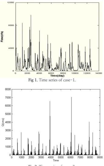
The case-1 series was analyzed for the investigation of its chaotic behavior by Kim et al. (1999) and it showed deterministic chaos. The case-1 series consists of 12,784 measurements
Fig 1. Time series of case-1.
Fig 2. Time series of case-2.
Table 1. Basic statistics of each time series
Case-1 Case-2
Mean 987.5548 (cfs) 66.1459 (cms) Standard deviation 1166.2364 205.1937
Max Value 10700 (cfs) 7062.6 (cms)
Min Value 5.6 (cfs) 0 (cms)
Skewness coefficient -0.1918 -0095
from January 1, 1954 to December 31, 1988. Another data set used consists of 8,776 measurements from January 1, 1974 to December 31, 1997. The time series plots are shown in Figs. 1 and 2, and basic statistics in Table 1.
2.2 Phase space reconstruction
The first step in the search for a deterministic behavior of underlying system is to reconstruct the dynamics in phase space.
The phase space can be approximated by using a single record of some observable x
t, t 1 , 2 , , N , where N is data size (Packard et al., 1980; Takens, 1981). A single value time series can reconstruct the attractor on m -dimensional phase space using delay method. The method entails the form of construction:
} ,
, , ,
{ x t x t x t 2 x t ( m 1 ) (1)
where is the delay time.
In streamflow series at St. Johns river near Cocoa, the autocorrelation function decays exponentially, selecting delay time at which autocorrelation function drops 1/e (Tsonis and Elsner, 1988). Thus, the delay time of streamflow series at St. Johns river near Cocoa is 48 days. In the case of inflow series at Soyang reservoir, the delay time = 10 days is chosen from the local minimum of autocorrelation function (Holzfuss and Mayer-Kress, 1986; Graf and Elbert, 1990). The attractors for the time series of case-1 and case-2 are reconstructed in 2-dimensional phase space as shown in Figs. 3 and 4.
Fig 3. Attractor for case-1.
Fig 4. Attractor for case-2.
2.3 Correlation dimension
After the attractor has been reconstructed using Eq. (1), quantitative properties of the chaotic system can be determined.
The correlation dimension introduced by Grassberger and Procaccia (1983) is widely used in many fields for the quantitative characterization of strange attractors. The correlation integral for the embedded time series is the following function:
M j i
j
i
x
x M r
r M N m C
)
11 ( ) 2 , ,
(
, r>0 (2)
Where, a ( ) 0 if a 0 , a ( ) 1 if a 0
N is the size of the data set, M N ( m 1 ) is the number of embedded points in m -dimensional space and || || denotes the sup-norm. C ( m , N , r ) measures the fraction of the pairs of points x
i, i = 1,2, ..., M , whose sup-norm separation is no greater than r . If the limit of C ( m , N , r ) as N exists for each r , we write the fraction of all state vector points that are within r of each other as C ( m , r ) = lim C ( m , N , r )
N
and the correlation dimension is defined as ( ) lim [log ( , ) / log ]
2
m
0C m r r
D
r. In
practice, N remains finite, and thus, r cannot go to zero; instead, a linear region of slope D
2( m ) can be found in the plot of
) , , (
log C m N r vs. log r. The slope, D
2( m ) or is correlation dimension which can be calculated from the following equation :
i i
i i i
r r
r m C r
m Slope C
] log[
] log[
)]
, ( log[
)]
, ( : log[
1 1
(3)
Common least squares methods are not optimal for use when the data points are not independent. Therefore, we may use Eq. (4) for the calculation of correlation dimension because the individual increments of the correlation integral are independent (Barnett, 1993).
Ni i i
N
i i i i i
x x
y y x x
2
1 2
2 1 1
) (
) )(
(
(4)
Where, x = log( r ) and y = log[C( m , r )].
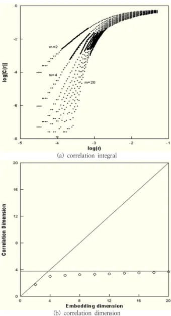
(a) correlation integral
(b) correlation dimension
Fig. 5. Estimation of correlation dimension for case-1.
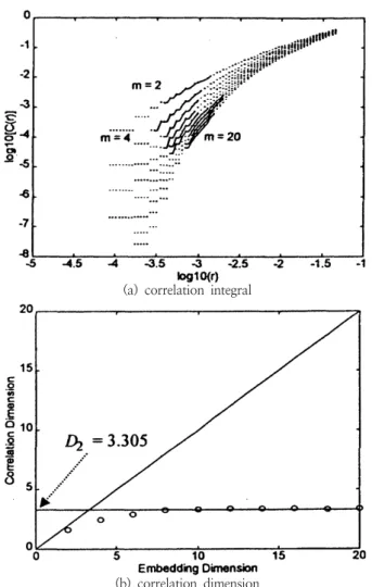
It is possible to say that the time series has a chaotic characteristic (Kim et al., 1999). For the time series of case-1 and case-2, the linear regions of the correlation integrals are visually chosen from Figs. 5(a) and 6(a). The linear regions are shown as dark lines and the correlation dimensions are calculated as shown in Figs. 5(b) and 6(b). Streamflow series at St. Johns river near Cocoa shows the correlation dimension of 3.305
On the other hand, in the case of inflow series at Soyang
reservoir, the correlation dimension calculated is increasing
as embedding dimension is increased and it may be difficult
to conclude that the inflow series is chaos.
(a) correlation integral
(b) correlation dimension
Fig. 6. Estimation of correlation dimension for case-2
3. Forecasting Streamflow Using Chaotic Dynamics
3.1 DVS algorithm
For a scalar time series { x
i}= x
1, x
2,, x
N, the DVS algorithm attempts to fit models of the form:
) ,
, ,
(
( 1)T
i i i mi
f x x x
x (5)
It is used a least-squares method to find the function f that gives the best prediction for x
iTin the sense that the function minimizes the squared error within the model class. The integers T and m define the following quantities.
T : lead time or prediction horizon (prediction time into the future)
m : embedding dimension or dimension of the reconstructed phase space(number of taps of the tapped delay line)
Furthermore, the m are combined in the delay vector x
i. Here assuming equal spacing of the taps of the delay line,
i.e., x
iT f ( x
i, x
i, , x
i(m1)) , where is the lag time or lag spacing between each of the taps. After these definitions, the DVS algorithm is given by
(1) Normalize the time series to zero mean and unit variance.
(2) Divide the time series into two parts:
1) a training set or fitting set { x
1,…, x
Nf} used to estimate the coefficients of each model,
2) a test set or out-of-sample set { x
Nf+1,…, x
Nf+Nt} used to evaluate the model. Nf denotes the number of points in the fitting set, Nt the number of points in the test set.
(3) Choose T and m
(4) Choose a test delay vector x
ifor a T-step-ahead forecasting task ( i>Nf ).
(5) Compute the distances d
ijof the test vector x
ifrom the training vectors x
j(for all j such that ( m -1) < j < i – T ) (6) Order the distances d
ij(7) Find the k nearest neighbors x
(j1)through x
(kj )of x
i, and fit an affine model with coefficients , …, of the following form
mn l
n j n l
T
j
x
x
1 ) (
) 1 ( 0
)
(
, l=1, …, k.
) 1 ( )
1 (
2 m k N
f T m (6)
(8) Use the fitted model from step (7) to estimate a T -step-ahead forecast x
iT(k )
starting from the test vector, and compute its error
T i T i T
i
k x x
e
( )
(7)
(9) Repeat step (4) through (8) as ( i + T ) runs through the test set, and compute the mean absolute forecasting error
Nt Ti t
T i
m
N
k k e
E
1 ) (
) ) (
( (8)
Vary the embedding dimension m , and plot the curves E
m( k ) as functions of the number of nearest neighbor ( k ). Such a plot of the family of curves is called DVS plot.
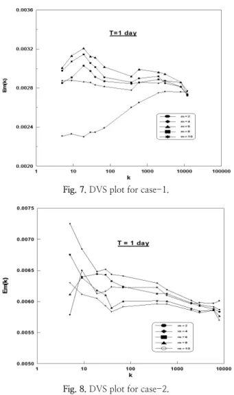
The name of above algorithm derives from the fact that the
shapes of the resulting plots can provide evidence of low
dimensional deterministic chaos, or of high dimensional or
stochastic dynamics. Low dimensional chaos is typically
characterized by U-shaped or monotonically increasing plots
whose minimum E
m( k ) values are small and occur at low values
of k . High dimensional or stochastic behavior is often indicated
Fig. 7. DVS plot for case-1.
Fig. 8. DVS plot for case-2.
by relatively large minimum E
m( k ) values occurring at high k values (Casdagli, 1991).
The DVS algorithm suggested by Casdagli (1991) is used for two flow series. The dimension of the reconstructed phase space m is varied from 2 to 10. Figs. 7 and 8 are the DVS plots for lead time T =1day. The daily streamflow series at St. Johns river near Cocoa has a chaotic characteristic and daily inflow series at Soyang reservoir has no chaotic.
Based on chaotic analysis, we may know daily streamflow at St. Johs river near Cocoa has the low E
m( k ) in DVS plot. However, the shape of DVS plot for daily inflow series at Soyang reservoir is a stochastic process. Thus, daily inflow series at Soyang reservoir does not have a chaotic characteristic.
The results of the DVS plots show the best k and m . Based on the local linear approximation method (Farmer and Sidorowich, 1987) with the best k and m , the forecasting is performed. The DVS algorithm has 301 days test sets of two daily flow series. The remaining data series are training sets.
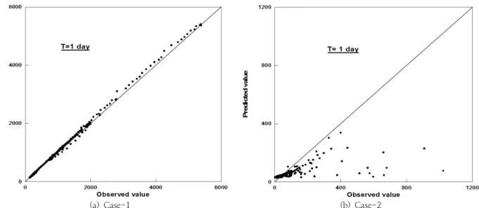
Because the DVS algorithm makes the relationship among the peak flows and among the low flows, the effect of the magnitude of data sets for forecast error may be small. Figs. 9 and 10 show the relationship between the observed and the forecasted values for each lead times ( T =1, 10, 20days). Tables 2 and 3 show the comparison of mean, standard deviation, peak, peak time and volume between the observed and the forecasted values for two series of case-1 and –2. Also, Tables 2 and 3
Table 2. Forecasting results based on DVS algorithm for case-1.
Observed T = 1 day T = 10 day T = 20 day
mean (cfs) 1110.0166 1118.9598 1182.3164 1312.8778
standard dev. 1172.8175 1188.1831 1181.7981 1247.1936
peak (cfs) 5390 5380.3591 4588.9906 5436.7147
peak time (day) 3 1 8 6
volume (ft3) 2.887*1010 2.910*1010 3.075*1010 3.414*1010
AMB 24.5945 232.8725 433.6558
RMSE 40.0200 356.4302 593.7325
RRMSE 0.0248 0.2209 0.3680
MRE 0.0266 0.2464 0.5782
correlation coef. 0.9995 0.9560 0.8951
Table 3. Forecasting results based on DVS algorithm for case-2
Observed T = 1 day T = 10 day T = 20 day
mean (cms) 78.2837 80.6159 54.2741 52.5867
standard dev. 131.1263 116.3670 55.3625 41.3863
peak (cms) 1023.5 901 454 325
peak time (day) 64 65 74 84
volume (m3) 2.036*109 2.100*109 1.408*109 1.365*109
AMB 40.2272 59.8196 62.5980
RMSE 106.9739 136.6363 135.5353
RRMSE 0.7013 0.8958 0.8886
MRE 0.5241 0.9006 1.1712
correlation coef. 0.6312 0.1436 0.1056
show the measures of forecast errors which can measure the forecast accuracy. As the forecast errors (AMB (Absolute Mean Bias), RMSE (Root Mean Square Error), RRMSE (Relative Root Mean Square Error, MRE (Magnitude of Relative Error)) are decreased, the correlation coefficient is approached to 1.
The chaotic streamflow time series shows that the correlation coefficients between the forecasted and the observed values are 0.9995 and the non-chaotic streamflow time series shows 0.6311 for 1 day-ahead lead time (see Tables 2 and 3, and Fig. 9). As the lead time is increased the accuracy of the forecast is decreased. Chaotic streamflow at St. Johns river near Cocoa, shows more accurate than non-chaotic inflow in their correlation coefficients and low forecasting errors (AMB, RMSE, RRMSE, MRE). The forecasting results of the lead time of 10, 20 day-ahead for chaotic streamflow are also relatively satisfactory.
3.2 Neural network