한국정보통신학회논문지 Vol. 23, No. 5: 495~507, May 2019
암시적 피드백 데이터의 행렬 분해 기반 누락 데이터 모델링
기가기1·정영지2*
Missing Data Modeling based on Matrix Factorization of Implicit Feedback Dataset
Ji JiaQi1 · Yeongjee Chung2*
1Lecturer, Department of Information Center, Hebei Normal University for Nationalities, ChengDe 067000, China
2*Professor, Department of Computer and Software Engineering, Wonkwang University, Iksan 54538, Korea
요 약
데이터 희소성은 추천 시스템의 주요 과제 중 하나이다. 추천 시스템에서는, 일부분만 관찰된 데이터이고 다른 부 분은 데이터가 누락된 대용량 데이터를 포함하고 있다. 대부분의 연구에서는, 데이터 세트에서 무작위로 데이터가 누락되었다고 가정하고, 관찰된 데이터만을 사용하여 추천 모델을 학습함으로써 사용자에게 항목을 추천하고 있다.
그러나, 실제로는 누락된 데이터는 무작위로 손실되었다고 볼 수 없다. 본 연구에서는, 누락 된 데이터를 사용자적 관 심의 부정적인 예라고 간주하였다. 또한, 3가지 샘플 접근 방식을 SVD++ 알고리즘과 결합하여 SVD++_W, SVD++_R 그리고 SVD++_KNN 알고리즘을 제안하였다. 실험결과를 통하여, 제안한 3가지 샘플 접근 방식이 기존 의 기본적인 알고리즘 보다 Top-N 추천에서 정확성과 회수율을 효과적으로 향상시킬 수 있다는 것을 보였다. 특히, SVD++_KNN 가 가장 우수한 성능을 보였는데, 이는 KNN 샘플 접근 방식이 사용자적 관심의 부정적인 예를 추출하 는데 가장 효율적인 방법이라는 것을 보여주었다.
ABSTRACT
Data sparsity is one of the main challenges for the recommender system. The recommender system contains massive data in which only a small part is the observed data and the others are missing data. Most studies assume that missing data is randomly missing from the dataset. Therefore, they only use observed data to train recommendation model, then recommend items to users. In actual case, however, missing data do not lost randomly. In our research, treat these missing data as negative examples of users’ interest. Three sample methods are seamlessly integrated into SVD++
algorithm and then propose SVD++_W, SVD++_R and SVD++_KNN algorithm. Experimental results show that proposed sample methods effectively improve the precision in Top-N recommendation over the baseline algorithms. Among the three improved algorithms, SVD++_KNN has the best performance, which shows that the KNN sample method is a more effective way to extract the negative examples of the users’ interest.
키워드 : 추천 시스템, 행렬 분해, 누락 데이터, 데이터 희소성
Keywords : Recommender System, Matrix Factorization, Missing Data, Data Sparsity
Received 11 March 2019, Revised 18 March 2019, Accepted 26 March 2019
* Corresponding Author Yeongjee Chung (E-mail: [email protected], Tel:+82-63-850-6887)
Professor, Department of Computer and Software Engineering, Wonkwang University, Iksan, 54538 Korea
Open Access http://doi.org/10.6109/jkiice.2019.23.5.495 print ISSN: 2234-4772 online ISSN: 2288-4165 Communication Engineering
Ⅰ. Introduction
The classic collaborative filtering recommender algorithms use user-item rating matrix to train recommendation model[1], then predicts user behavior and generates recommendation results. However, the rating matrix is generally sparse[2], which is a major problem for recommender algorithms. Data sparsity is mainly reflected the fact that each user has ratings on only a few items and each item has ratings only by a few users. For instance, Netflix dataset contains 480189 users rating on 17770 items and a total of 100480507 rated data, it shows that the data density is 100480507 / (480189*
17770) =1.18% and 1-1.18%=98.2% of the data is missing data; Movielens 100K dataset contains 943 users rating on 1682 items and a total of 100000 rated data, therefore the data density is 100000/(943*1682)
=6.3% and 1-6.3%=93.7% of the data is missing data.
The large amounts of missing data have made it difficult to select and design recommender algorithms. Most of the proposed algorithms train the model based on the sparse rating matrix [3-5]. These algorithms are often based on a potential assumption that the missing data is random. If this hypothesis is true, then the training model can make unbiased estimates based on existed data. However, the missing data is not random[6, 7], because if an item is a very popular item and has obtained a very high average rating from other users, then the active user will have a high probability to give this item a rating[8] and vice versa. Therefore, these models can’t describe the features of users and items without bias and can be improved.
In a typical recommender system application scenario, the user can select the items autonomously and rate on items by their preference[9]. For example, in an e-commerce application, users tend to rate their purchased items; on the movie website, users will give comments and ratings on films they’ve already seen. With a large number of unfocused, uninterested items or movies on the website, users rarely buy or watch deliberately, nor do they give a rating. It can be considered that these
missing data is the user’s subjective unwillingness to rate. Therefore in this paper we think that missing data in recommender system is not a random missing. We believe that missing data is the data that users are not willing to rate and these data can serve as a negative example of user’s preference.
For any user, all items are divided into two sets. One set are positive examples (marked as set+) of user’s preference, a collection of items that the user wants to rate. The other set are negative examples (marked as set-) of users’ preference, a collection of items that the users don’t want to rate. In recommender system, rating data in rating matrix is part of set+, the set- and the rest part of set+ constitutes the missing data together. The goal of the recommender algorithm is to identify the part of the missing data belonging to the set+ and recommend it to users. But there is a great difficulty accomplishing this goal that we can obtain positive examples from rating matrix, however it is lack of explicit negative examples in rating matrix. In this case, the model cannot be trained effectively. Fortunately, these negative examples are not nonexistent, but are hidden in missing data. If the negative examples can be identified from the missing data effectively, and then we use these identified negative examples to combine with positive example to train the model together, the missing positive examples can be found and recommend them to users.
In view of the above problems, weighted method, random sample method and K-Nearest neighbor sample method are proposed to set up models for missing data.
The details of the proposed method will be described in the next section. These are three general methods and can be used in all kinds of collaborative filtering algorithms to improve the recommendation performance.
Ⅱ. Modeling of Missing Data
In recommender systems, users are free to choose items and rate on them. A survey in literature [10] shows that 93.9 percent of users regularly rate on their favorite
items and only 36.5 percent of users regularly rate on items they feel generally. The background of the survey is Yahoo’s music site, and rated object is the type of song-based music items. This kind of item is mostly 3-5 minutes long and often free to listen to. So it has features of less time cost and being free. In this case, the cost of listening and rating are relatively small as well. Even so, only a small number of users are willing to rate score on items they feel generally. If the scene is switched to the background of high fee (commerce) or time cost (watching movies), there will be smaller percentage of users who will rate on items they feel generally. It can be inferred that the user rating behavior of the recommender system is the embodiment of user’s choice tendency and the embodiment of user’s interest. As described in the previous section, for any user, we classify the items which we are interested in or willing to rate into the set set+; we classify the items which we aren’t interested in or unwilling to rate into the set set-. The data in set+ are positive examples of users’ interest and the data in set- are negative examples of users’ interest. The data in rating matrix is part of positive examples, the missing part of the positive examples and negative examples constitute the missing data together.
The goal of recommender algorithm is to identify unrated positive examples from missing data, then recommend high rated items in these positive examples to users [11]. However, due to the fact that there are only positive examples in the rating matrix, it is very difficult for the recommendation model to distinguish the positive and negative examples by only using the rating matrix data. Therefore, this section proposes a method for modeling missing data to obtain negative examples.
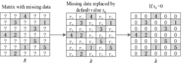
Since positive and negative examples are two different sets, their rating values should also be in two different ranges. The rating range for positive examples of typical recommender system is 1-5, so we define a default value rn = 0 for negative examples. In this case, we can represent positive examples and negative examples in a same rating matrix and the range of value change to 0-5 (the value of positive examples is greater than 0 and the
value of negative examples is equal to 0). The effect of different values rn on recommender system will be analyzed by later experiments.
2.1. Weighted Method
Underlying the proposed weighted method, it is considered that the missing data are negative examples to some extent. But these negative examples are not provided by the user explicit. Therefore, when the missing data are positive examples, the confidence is high. By contrast, when the missing data are negative examples, the confidence is very low. The weighted method describes the difference in confidence by adjusting the weights of different data in the recommended model. The weight calculation method is shown in Eq.(1).
∉ ∈ (1) Where is the rating matrix, is the weight of user rating on item . If is not missing data then the weight is 1, otherwise the weight is . is a parameter predefined global weighted value for missing data, the range of should be [0,1].The weighted method uses as the default rating of missing data, so as to describe user rating data and missing data in a same matrix. Therefore we re-define
as which is described in Eq.(2)
∈ ∉ (2) At this time, instead of becomes the element of the rating matrix . Obviously, contains two parts, one is which is the original value in the rating matrix , and another one is which is the missing value in the rating matrix . This conversion process can be shown in Fig. 1.Fig. 1 Replacement of missing data with
After the weighted method is applied, the optimization objective of the recommender algorithm is minimizing the weighted loss function as is described in Eq(3).
∙ (3)
Where is a unified data model constructed by weighted method. is a matrix and can be seen in Fig. 1 (middle or right picture). is an element of , is the rating value predicted by user for item . The weighted method can be combined with the traditional collaborative filtering recommendation algorithm such as user-based CF, item-based CF or SVD++[12]. Then the training process of the recommendation algorithm is adjusted to improve the recommendation performance based on the Eq. (3).
2.2. Random Sample Method
The experimental results in later section show that the weighted method can improve the recommendation performance effectively; however it still has two main problems: (1) The weighted method considers that all the missing data are negative examples to some extent, but in fact there are some positive examples in these data. (2) The raw data are sparse, but after using weighted method the data are dense. In this case, the computational complexity of model training increases dramatically. In order to alleviate these problems, we propose an approach for modeling missing data using random sample method and obtaining negative examples.
Compared with weighted method, the proposed approach randomly extracting part of the data from the missing data as negative examples can reduce the computational
complexity effectively.
In this section, we consider that part of the missing data are negative examples, therefore we use random algorithm to extract a certain proportion of data from missing data as negative examples. is used to indicate the proportion of extraction and the extracted dataset is denoted as . together with form a unified data model ∪. The elements in can be describe in Eq.(4).
∈∈ (4) Fig. 2 shows the conversion process from to.Fig. 2 Random replacement of missing data with
Random sample method requires data to train and optimize the recommender model. The size of the data has been fixed, so the computational complexity of the random sample method depends on the size of . When is 1, is a complete set of missing data, and the computational complexity of random sample method is equivalent to the weighted method; when the
is between ∼ , the smaller the is, the less volume of the data get, so the computational complexity is smaller.
In the random sample method, the selection of partial data from missing data combined with data R influences the training of recommender model. The random sample method only changes the training data source, and does not affect the recommendation model itself. In other words, the weight of random extracted data in is equivalent to the weight of data in . Therefore, after using the random sample method, the optimization goal
of the recommender algorithm is not multiplied by the weight . The formal description of the loss function is shown in Eq.(5)
(5)
It is important to note that random sample method obtains negative examples from missing data randomly, therefore it must exist random error in this process. In order to reduce the random errors caused by the random sample method, the random sample should be repeated in iteration during training.
2.3. K-Nearest Neighbor Sample Method
Random sample method can reduce the computational complexity effectively by using only partial missing data. However, the random sample method obtains the negative examples from the missing data randomly, it makes that the missing positive examples and the negative examples have equal probability of being sampled. In order to reduce the probability of missing the positive examples being sampled and increase the probability of missing the negative examples being sampled, -Nearest neighbor[13] sample (KNN sample) method is proposed to solve this problem.
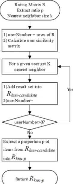
The KNN sample method assumes that if a user’s nearest neighbor doesn’t rate on an item, the user won’t rate on that item with high probability. Therefore, for any user, user similarity should be calculated. The process of KNN sample method can be described like this. (1) The first step is to calculate user similarity matrix; (2) The second step is to find k nearest neighbor for a given user; (3) The third step is to obtain a set in which the item has not been rated by the active user nor by the user’s neighbors, then add the set into
which is a candidate set for negative examples; (4) The fourth step is to repeat (2)-(3), after that, extract a certain proportion of items from
as the negative examples and represent as
. Fig. 3 shows this process.
Fig. 3 Flow chart of K-Nearest neighbor sample method
By KNN sample method, we can obtain a set of
and each item in is a negative example with high probability. The unified data model can be represented as ∪ and the elements in is described in Eq. (6)
∈∈ (6) Same with using random sample method, the loss function (same with Eq.(5)) is no need to multiply the weight . But there are two points different from random sample method: (1) the data in are different, is random sample using random sample method, however is based on K-Nearest neighbor using KNN sample method. (2) KNN sample method doesn’t need re-sample in iteration during training.
Ⅲ. Recommendation Algorithm
Section 2 introduces a series of methods for modeling missing data by weighting or sampling. These methods can be combined with various collaborative filtering
recommendation algorithms to help solve the problem of data sparsity and improve the recommendation effect.
This section uses the SVD++ algorithm as the original recommendation algorithm, combined with missing data modeling method introduced in section 2 to improve the performance of Top-N recommendation.
SVD++ refers to a matrix factorization model which makes use of implicit feedback information. In general, implicit feedback can refer to any kinds of users' history information that can help indicate users’ preference. The SVD++ model is formally described as following equation:
∈
(7)
Where is the overall average rating, the parameters
and indicate the observed deviations of user and item , respectively, from the average . and are user-factors vector and item-factors vector respectively.
contains all items for which provided an implicit preference. is a factor vector for item .
The SVD++ algorithm considers missing data as unknown information, training parameters on the rating matrix and learning model. We will improve the SVD++ algorithm by using the proposed missing data modeling method to improve its ability to utilize missing data, thus improving the recommendation performance.
3.1. Improved Algorithm Using Weighted Method In this section, we introduce an improved SVD++
algorithm using the weighted method, which is called as SVD++_W algorithm. SVD++ and SVD++_W use the same rating predict model which is defined in Eq.(7), but they use different data and loss functions.
Unlike SVD++ which uses only the data to train models, SVD++_W uses both data R and missing data which have been defined in Eq.(2). In addition, the loss function of SVD++_W is weighted, therefore the optimization objective should be adjusted to the form described in Eq(8).
min
∈
∈
∥
∥
∥
∥
∈
∥
∥
(8)
SVD++_W use the to train the model in order to minimize the weighted square error between prediction results and real results. The predict error is
. Then the parameters are adjusted by using descent gradient as follows:
←
←
←
←
∈
∀∈ ←
There are some problems in the above iteration process: (1) and indicate the observed deviations of user
and item , respectively, from the average , they represent the tendency of the user or product to score in the observed data. However in the , is used to indicate the missing data, but these ratings are not explicitly given by the user. Therefore the effect of missing data should not be considered when updating and . In addition, is a parameter that reflects the implicit feedback information and should not be affected by the missing data either. So we should not use the weight parameter when updating these three parameters but we should use the raw matrix R. For unified representation, we use another parameter
whose value is indicates is in and denotes
belong to the missing data.
∈ ∈ (10) The final training process is shown in Eq.(9)
← × × ×
← × × ×
← × × × ×
← × × ×
∈
×
∀∈ ← × × ×
× ×
After training, all parameters value can be obtained.
These parameter values are input into Eq.(7), and when giving a user and item , we can calculate the predicted rating of for .
3.2. Improved Algorithm Using Sample Method In this section, another improved SVD++ algorithm using sampling method is introduced. According to the different sample methods, the use of random sample method to improve the SVD++ is recorded as SVD++_R, using the K-nearest neighbor sample method to improve the SVD++ is known as SVD++_KNN.
The optimal objective and training procedures of SVD++_R and SVD++_KNN are same with SVD++_W which can be seen in Eq.(8) and Eq.(11). However the data is used in SVD++_R and SVD++_KNN are quite different from SVD++_W. As mentioned in the previous section, the data which is used by SVD++_R are defined by Eq.(4) and the data which is used by SVD++_KNN are described in Eq.(6). For the sake of completeness, the data, optimization goals, training procedures and prediction formula required for these two improved algorithms are listed respectively as follows:
(1) SVD++_R
Data matrix: . is the element of shown as follows:
∈ ∈ (12)Optimization goals:
min
∈
(13)
∈
∥
∥
∥
∥
∥
∥
∈
∥
∥
Training procedures:
← × × ×
← × × ×
← × × × ×
← × × ×
∈
×
∀∈ ← × × ×
× × Prediction formula:
∈
(15)
(2) SVD++_KNN
Data matrix:. is the element of shown as follows:
∈∈ (16) Optimization goals:min
∈
∈
∥
∥
∥
∥
∈
∥
∥
(17)Training procedures:
← × × ×
← × × ×
← × × × ×
← × × ×
∈
×
∀∈ ← ×
× ×
× × (11)
(14)
(18)
Prediction formula:
∈
(19)
Ⅳ. Experiment evaluation
4.1. Dataset and evaluation metrics
In this experiment the dataset of MovieLens 100k is used for experiment evaluation. It contains 100,000 ratings from 943 users on 1682 movies (each user has rated 20 or more movies). The dataset is divided into a training set and a test set. 80% of the data is used as training set, 10% of the data is used as validate set and 10% of the data is used as test set. Training set is used to train model, validate set is used to choose parameters and the test set is used to evaluate the performance of algorithm. We use 5-fold cross validation method to get the final experiment results.
4.2. Configuration
In order to verify the effect of the missing data modeling method and the corresponding recommendation algorithm proposed in this section, first we will compare the three algorithms (SVD++_W, SVD++_R, SVD++
_KNN), then compare this proposed algorithms with other baseline methods such as use-based CF, item- based CF and SVD++.
In order to compare and analyze the effect of the recommendation algorithms more effectively, we select the best performance parameters for the baseline algorithm through experiments. The parameter selection process is no longer described in the paper, and the corresponding parameters are listed below. Both Item-base CF and user-based CF use Pearson similarity to measure item similarity or user similarity respectively, and choose k=50 as nearest neighbors. For SVD++, we set regularization factor and learning rate . The algorithm (SVD++_W, SVD++_R, SVD++_KNN) uses the same regularization
factor and learning rate with SVD++ to reduce the impact of different parameters on the analysis of recommendation effect. In addition, the three improved algorithms add some new parameters, and the effects of these parameters on the recommendation effect are firstly analyzed. Then the proposed algorithm and the baseline algorithm are compared and analyzed.
4.3. Parameter analysis and choose
First, the influence of different parameter settings on the recommendation effect is analyzed through experiments according to the recommendation algorithm proposed in this chapter; then we find the optimal parameter. When the influence of parameters is analyzed, the accuracy of recommendation algorithm is mainly considered. In addition, when an algorithm contains multiple parameters, it is necessary to keep the other parameters unchanged when a parameter is analyzed.
(1) Choose Parameter for SVD++_W
SVD++_W is the improvement of SVD++ algorithm using weighted method. The algorithm contains two new parameters, and , where is the weight of missing data and is the default rating for missing data. We first fix then change to analyze the influence of recommendation performance by SVD++_W.
Fig. 4 shows the curve of precision of SVD++_W with different , where the value of increases from to
by step . When , equivalent to all missing data does not have any effect on the training process, in this case SVD++_W degraded to SVD++. When is
or , the precision of SVD++_W is much better than SVD++. This indicates that using weighted method to model negative examples in missing data can improve the precision of SVD++ algorithm effectively. However, when is greater than or equal to , the precision of SVD++_W is no longer superior to the SVD++. This shows that the confidence level of missing data as negative example is too large, which is not conducive to enhancing the ability of SVD++ algorithm to recommend related items, and it is also shown that all missing data
are inappropriate as negative examples. On the whole, when is , the precision of SVD ++_W is highest, so we select as missing data weight.
Fig. 4 The curve of precision when and is changed
Now we fix and change from to increased by step 1 to observe the precision curve. From Fig. 5 we can see when , the precision is the highest. But with the further reduction of , the accuracy is also reduced. This is because the confidence level of missing data as negative examples is low, and the lower default rating will make the recommendation model shift to the negative examples
Fig. 5 The curve of precision when and is changed
(2) Choose parameter for SVD++_R
SVD++_R is the improved SVD++ algorithm using random sample method described in the previous. The algorithm contains two additional parameters and .
is the ratio of randomly selected negative examples from missing data; is the default value for missing data. First, we will analyze the impact of different on the recommendation effect of SVD++_R algorithm.
Similar to those mentioned earlier, we fix and change .
Fig. 6 The curve of precision when and is changed
Fig. 6 shows the precision curve of SVD++_R with the change of . The value of increases from 0 to 1, with 0.1 as step size. When is 0, SVD++_R does not need to select negative examples from missing data, so SVD++_R degenerates to SVD++. When is 0.1 or 0.2, the precision of SVD++_R is better than SVD++. This shows that using random sample method to extract negative examples from missing data, and use these negative examples and observation data together to train the recommendation model, can improve the performance of Top-N recommendation effectively. However, when
is greater than or equal to 0.3, the precision of SVD++_R is no longer better than SVD++, it indicates that if too many data are extracted from missing data as negative examples, it is not conducive to enhancing the ability to recommend related items. This is mainly
because the missing data contain negative examples and un-rating positive examples, and random sample makes the positive and negative examples extracted in same ratio, however all the data extracted by SVD++_R as negative examples, which makes error data to be included in the training model, and error data ratio will increase with the increase of the sample proportion.
When the side effect of the error information on the recommendation model is greater than the benefit of the new negative example information to the recommendation model, the improvement SVD++ algorithm will gradually decline with the random sample method. It can be seen from Fig. 6 that when is 0.2, SVD++_R gets the best recommendation effect. Therefore, we choose as the ratio of negative examples in missing data.
We fix and change from -5 to 0 to observe the change of precision. From Fig. 7 we can see when
the precision of SVD++_R is the highest. This shows that the default rating for the extracted data is not the-lower-the-better, but it should be treated as negative examples.
Fig. 7 The curve of precision when and is changed
(3) Choose parameter for SVD++_KNN
SVD++_KNN is the improved SVD++ algorithm using k-nearest neighbor sample method described in the previous. The algorithm contains three additional parameters , and . Where is the number of
nearest neighbors; is the ratio of randomly selected negative examples from missing data; is the default value for missing data. So, the negative examples in SVD++_KNN are determined by and .
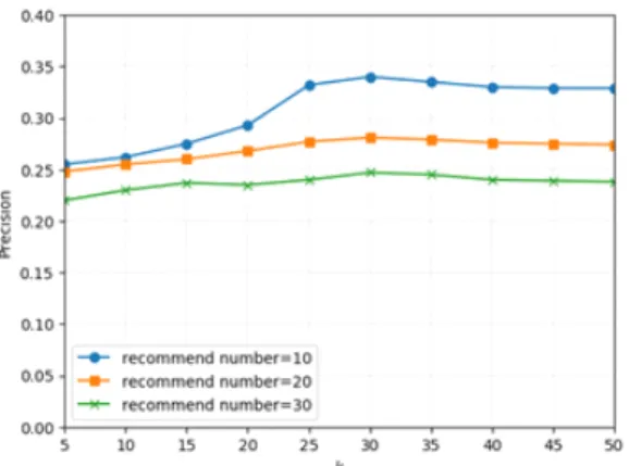
In order to analyze the influence of different parameters on SVD++_KNN, first we fix , and change k from 5 to 50 increased by step 5. Fig. 8 illustrates that when k is 30, the precision is the highest.
Fig. 8 The curve of precision when , and is changed
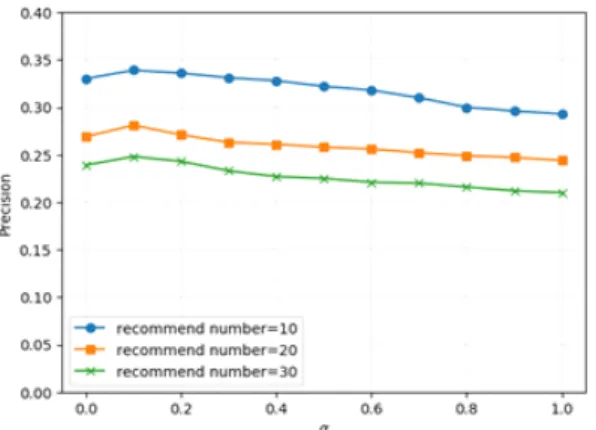
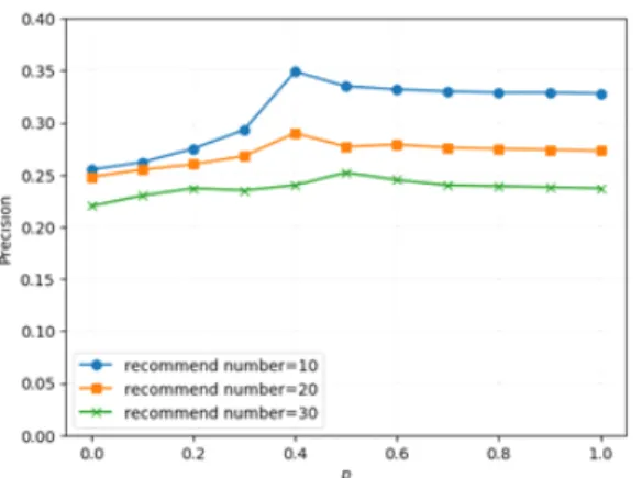
Second, we fix , and change from 0 to 1. Fig. 9 shows the result. When is 0, SVD++_R degenerates to SVD++. No matter what the value of p, the precision of SVD++_KNN is better than SVD++.
This phenomenon is completely different from SVD++_W and SVD++_R. The main reason is that SVD++_KNN uses k-nearest neighbor sample method which is using the behavior of similar users to increase the sample probability of negative examples greatly, and reduce the sample probability of positive example. This process guarantee the confidence of the negative examples obtained from the sample.
Fig. 9 The curve of precision when , and
is changed
Fig. 10 The curve of precision when , and
is changed
We can see that when recommender number is 10 or 20, we obtain the highest precision at , but when recommender number is 30, we get the highest precision at . Considering that the real system won’t recommend items more than 20 in practice generally, so we decide to choose as the best parameter.
At last, we fix and change from
to 0. Fig. 10 shows that the precision is highest when
Based on the above analysis, the results of the final parameter selection are listed in Table 1. The proposed algorithm will be based on these parameters to compare with other algorithms in the next section.
Table. 1 Parameter selection result
Proposed algorithm Selected parameter
SVD++_W
SVD++_R
SVD++_KNN
4.4. Experimental results
This section compares the proposed algorithm with the baseline from the aspects of precision, recall, F1 and coverage. From Table 2 to Table 4 the experimental results are listed with different recommender number.
We can infer that whatever the recommender number is, the performance of SVD++_KNN is the best.
Table. 2 Experimental result when recommender number is 10
Algorithm Precision Recall F1 coverage BaseLine Item-based
CF
0.3124 0.1478 0.2007 0.2191
User-based CF
0.3218 0.1523 0.2067 0.1261
SVD++ 0.3298 0.1560 0.2118 0.1310 Proposed
approach
SVD++_W 0.3402 0.1598 0.2174 0.1298 SVD++_R 0.3501 0.1601 0.2197 0.1450 SVD++_K
NN
0.3601 0.1608 0.2223 0.2304
Of all the indicators, we are most concerned with precision. Where SVD++_KNN is the best, followed by SVD++_W and SVD++_R.
Table. 3 Experimental result when recommender number is 20
Algorithm Precision Recall F1 coverage BaseLine Item-based
CF
0.2593 0.2454 0.2522 0.3543
User-based CF
0.2574 0.2436 0.2503 0.1871
SVD++ 0.2699 0.2554 0.2625 0.1894 Proposed
approach
SVD++_W 0.2812 0.2591 0.2697 0.1876 SVD++_R 0.2901 0.2632 0.2760 0.1932 SVD++_K
NN
0.3032 0.2692 0.2990 0.3590
Table. 4 Experimental result when recommender number is 30
Algorithm Precision Recall F1 coverage BaseLine Item-based
CF
0.2255 0.3200 0.2646 0.4273
User-based CF
0.2206 0.3131 0.2588 0.2354
SVD++ 0.2306 0.3273 0.2706 0.2311 Proposed
approach
SVD++_W 0.2480 0.3298 0.2831 0.2561 SVD++_R 0.2530 0.3336 0.2887 0.2401 SVD++_K
NN
0.2600 0.3391 0.2943 0.4306
This illustrates that the algorithm proposed in this chapter has a high Top-N recommendation precision.
These three algorithms based on missing data modeling are improved SVD++ algorithm. The good performance verifies the existence of negative examples in the missing data and validity of the corresponding missing data modeling method. In addition, the performance of SVD++_KNN is slightly better than SVD++_W and SVD++_R, it explains that using the nearest neighbor sample method to obtain negative examples is a more effective method for missing data modeling.
In summary, the three improved algorithm proposed in this chapter are better than baseline algorithms. The experimental results validate the view that the missing data contains negative examples of user interest, and the effectiveness of weighted method, the random sample method and the k-nearest neighbor sample method for missing data modeling. Among the three improved algorithms, SVD++_KNN has the best performance, which shows that the k-nearest neighbor sample method is a more effective way to extract the negative examples of the user’s interest.
Ⅴ. Conclusions
In order to deal with data sparsity problem, we think that missing data do not lose in randomly. In actually, parts of missing data should regard as user unwilling to
rate on the items, and treat these missing data as negative examples of users’ interest. To cope with this challenge, three approaches using negative examples for modeling missing data are proposed: weighted method, random sample method, k-nearest neighbor sample method.
After that these approaches are seamlessly integrated into SVD++ algorithm and then propose SVD++_W, SVD++_R and SVD++_KNN algorithm for enhancing the Top-N recommendation performance. In the experiments parts, the parameters selection process is discussed in detail and the final results show that our proposed approaches significantly improve the precision for Top-N recommendation.
ACKNOWLEDGEMENT
This paper was supported by Wonkwang University in 2019.
REFERENCES
[ 1 ] V. Bajpai, and Y. Yadav, “Survay Ppaer on Dynamic Recommendation System for e-Commerce,” International Journal of Advanced Research in Computer Science [Online], vol. 9, no. 1, pp. 774-777, 2018. Available:
http://www.ijarcs.info/index.php/Ijarcs/article/view/5503/4 595
[ 2 ] I. E. Kartoglu, and M. W. Spratling, “Two collaborative filtering recommender systems based on sparse dictionary coding,” in Knowledge and Information Systems, vol. 57, no.
3, pp. 709-720, 2018.
[ 3 ] W. Lu, F.-l. Chung, K. Lai, and L. Zhang, “Recommender system based on scarce information mining,” Neural Networks, Elsevier, vol. 93, pp. 256-266, 2017.
[ 4 ] H. S. Moon, J. H. Yoon, and J. K. Kim, “The impact of information amount on the performance of recommender systems,” in Proceedings of the 18th Annual International Conference on Electronic Commerce(ICEC 2016):
e-Commerce in Smart connected World, Suwon, Republic of Korea: ACM New York, NY, Article no. 6, 2016.
[ 5 ] R. Heckel, and K. Ramchandran, “The Sample Complexity of Online One-Class Collaborative Filtering,” Machine
Learning (cs.LG) arXiv preprint arXiv:1706.00061, 2017 [Online]. Available: https://arXiv.org/abs/1706.00061.
[ 6 ] I. Jordanov, N. Petrov, and A. Petrozziello, “Classifiers Accuracy Improvement Based on Missing Data Imputation,” Journal of Artificial Intelligence and Soft Computing Research(JAISCR), vol. 8, no. 1, pp. 31-48, 2018.
[ 7 ] D. Li, C. Miao, S. Chu, J. Mallen, T. Yoshioka, and P.
Srivastava, “Stable Matrix Approximation for Top-N Recommendation on Implicit Feedback Data,” in Proceedings of the 51st Hawaii International Conference on System Sciences(HICSS-51), Waikoloa Village, HI: HICSS, pp.
1563-1572, Jan. 2018.
[ 8 ] X. Zhao, Z. Niu, K. Wang, K. Niu, and Z. Liu, “Improving top-N recommendation performance using missing data,”
Mathematical Problems in Engineering [Online], vol. 2015, Article ID 380472, 2015. Available: https://www.hindawi.com/
journals/mpe/2015/380472/
[ 9 ] M. H. Abdi, G. O. Okeyo, and R. W. Mwangi, “Matrix Factorization Techniques for Context-Aware Collaborative Filtering Recommender Systems: A Survey,” Computer and Information Science, Canadian Center of Science and Education, vol. 11, no. 2, pp. 1-10, 2018.
[10] B. Marlin, R. S. Zemel, S. Roweis, and M. Slaney,
“Collaborative filtering and the missing at random assumption,” Machine Learning (cs.LG) arXiv preprint arXiv:1206.5267, 2012 [Online]. Available: https://arXiv.org /abs/1206.5267.
[11] D. Jannach, and G. Adomavicius, “Recommendations with a purpose,” in Proceedings of the 10th ACM Conference on Recommender Systems, Boston, MA: ACM New York, NY, pp. 7-10, 2016.
[12] Y. Koren, “Factorization Meets the Neighborhood: a Multifaceted Collaborative Filtering Model,” in Proceedings of the 14th ACM SIGKDD International Conference on Knowledge Discovery and Data Mining. Las Vegas, NV:
ACM New York, NY, pp. 426-434, Aug. 2008.
[13] D.-K. Chae, S.-C. Lee, S.-Y. Lee, and S.-W. Kim, “On identifying k-nearest neighbors in neighborhood models for efficient and effective collaborative filtering,” Neurocomputing, Elsevier, vol. 278, pp. 134-143, 2018.
기가기(Ji JiaQi)
2007.7 Dept. of Computer Science and Technology, Nanchang University B.S., China 2010.1 Dept. of Computer Application Technology, Nanchang University M.S., China 2018.8 Dept. of computer Engineering, Wonkwang University , Ph.D., Korea
※관심분야 : Big Data Processing, Recommender System, Machine Learning
정영지(Chung, Yeongjee)
1995 ~ 원광대학교 컴퓨터·소프트웨어공학과 교수 1993 ~ 1995 한국전자통신연구원 선임연구원 1987 ~ 1993 삼성종합기술원 선임연구원 연세대학교 전기공학과 공학박사
※관심분야 : 컴퓨터 네트워크, 빅데이터 정보처리, 모바일 컴퓨팅