Modeling of CO₂ Emission from Soil in Greenhouse

Kor. J. Hort. Sci. Technol. 30(3):270-277, 2012 DOI http://dx.doi.org/10.7235/hort.2012.12082

Modeling of CO 2 Emission from Soil in Greenhouse

Dong Hoon Lee

, Kyou Seung Lee

, Chang Hyun Choi

, Yong Jin Cho

, Jong-Myoung Choi

, and Sun-Ok Chung

1

Department of Bio-Mechatronic Engineering, Sungkyunkwan University, Suwon 440-746, Korea

2

Department of Horticulture, Chungnam National University, Daejon 305-764, Korea

3

Department of Biosystems Machinery Engineering, Chungnam National University, Daejon 305-764, Korea

Abstract. Greenhouse industry has been growing in many countries due to both the advantage of stable year-round crop production and increased demand for fresh vegetables. In greenhouse cultivation, CO

concentration plays an essential role in the photosynthesis process of crops. Continuous and accurate monitoring of CO

level in the greenhouse would improve profitability and reduce environmental impact, through optimum control of greenhouse CO

enrichment and efficient crop production, as compared with the conventional management practices without monitoring and control of CO

level. In this study, a mathematical model was developed to estimate the CO

emission from soil as affected by environmental factors in greenhouses. Among various model types evaluated, a linear regression model provided the best coefficient of determination. Selected predictor variables were solar radiation and relative humidity and exponential transformation of both. As a response variable in the model, the difference between CO

concentrations at the soil surface and 5-cm depth showed are latively strong relationship with the predictor variables. Segmented regression analysis showed that better models were obtained when the entire daily dataset was divided into segments of shorter time ranges, and best models were obtained for segmented data where more variability in solar radiation and humidity were present (i.e., after sun-rise, before sun-set) than other segments. To consider time delay in the response of CO

concentration, concept of time lag was implemented in the regression analysis. As a result, there was an improvement in the performance of the models as the coefficients of determination were 0.93 and 0.87 with segmented time frames for sun-rise and sun-set periods, respectively. Validation tests of the models to predict CO

emission from soil showed that the developed empirical model would be applicable to real-time monitoring and diagnosis of significant factors for CO

enrichment in a soil-based greenhouse.

Additional key words: empirical model, real-time monitoring, regression analysis

*Corresponding author: [email protected]

※ Received 17 April 2012; Revised 16 May 2012; Accepted 22 May 2012. This research was supported by RDA (Rural Development Administration).We acknowledge contribution of Dr. Kenneth A. Sudduth, Agricultural Engineer, USDA-ARS, USA for proof reading and revision of the manuscript.

Introduction

There has been a tremendous growth of greenhouse industry in many countries due to both an increased demand for fresh vegetables and the need for stable year-round crop production.

Since CO

concentration plays an essential role in the photo- synthesis process of crops, optimum control of CO

enrichment based on accurate monitoring of added CO

in a greenhouse is necessary to improve the efficiency and profitability of crop production and to reduce environmental impacts that may influence global warming.

The environment of a greenhouse can be modeled as a nonlinear system with multiple coupled variables. Accurate monitoring of CO

concentration is the key to optimal control

of air fertilization by CO

enrichment in a greenhouse, but is complicated by a variety of factors such as temperature, humidity, and light intensity (Chen and Tang, 2010; Pohlheim and Heiβnet, 1991). Design and implementation of an effective control system for greenhouses requires continuous measurement of CO

concentration (Körnet et al., 2007).

Although many researchers investigated CO

control in a greenhouse, most of them focused on long term ecological research (Caetano et al., 2008) or the mathematical model of a non-soil based agricultural facility (Körnet et al., 2007;

Zhang et al., 2007). While many researchers have investigated

interactive relationships between the concentration of CO

in

the ambient air and crop growth, for example CO

exchange

of foliage plants (Park et al., 2010) and respiration affected

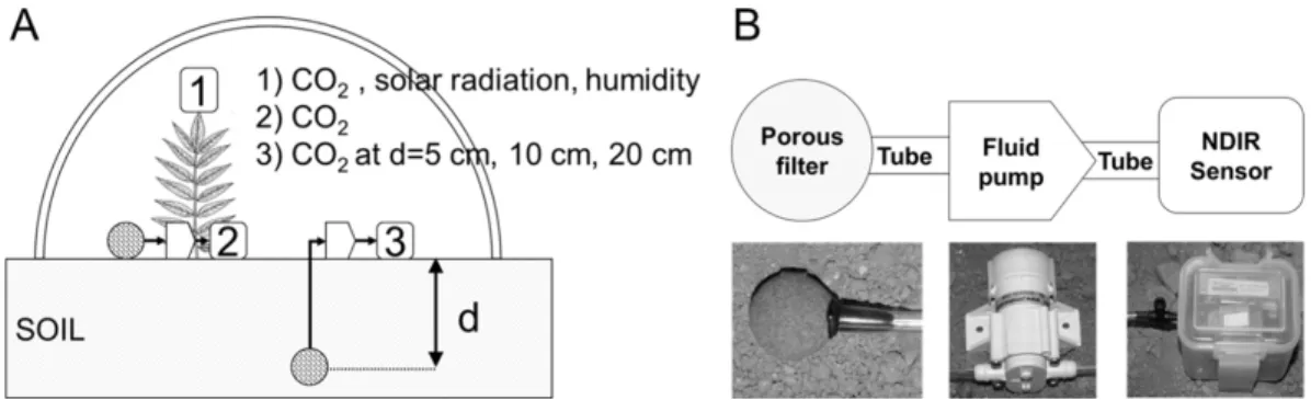
Fig. 1. Overall data collection scheme (A). Diagram explaining measurement of CO

concentration at different soil depths in the soil (B).

by CO

treatment (Jeong et al., 2006), more investigation of CO

interaction with soil would be useful.

In a soil-based greenhouse, there are generally three ways that CO

is supplied to the system. The traditional way is to supply CO

from the external ambient air by ventilation.

The second path is to enrich CO

using an air fertilization device, and the third path is to supply from the soil. Presence of these different pathways creates additional difficulty in accurate monitoring of ambient CO

concentration. Because CO

concentration in the ambient air inside the greenhouse would be considerably and quickly affected by any external supplement even in a short time, our assumption was that the level or change of CO

concentration in soil might give us information useful for real-time monitoring.

Because a standard method for real-time measurement of CO

emission from soil is not available, many researchers have reported time-dependent mathematical models for predicting CO

emission from soil (Jassal et al., 2004; Kabweet al., 2002; Lou et al., 2004; Ouyang and Zheng, 2000; Smart and Josep, 2005; Takahashi et al., 2004; Zhang et al., 2007).

For evaluation of their prediction models, reference values were determined using the closed chamber method (Camarda et al., 2009; DeSutter et al., 2006) or electrical sensors such as a solid fixation sensor (Tang et al., 2003) or an infrared gas sensor (Subke et al., 2003). In these studies, CO

emission was related to various environmental properties such as soil temperature (Fang and Moncrieff, 1999; Jassal et al., 2004), relative humidity (Granieri et al., 2003; Li et al., 2008;

Ouyang and Zheng, 2000), soil water content (Jassal et al., 2004; Maestre and Cortina, 2003), solar radiation (Ouyang and Zheng, 2000), and soil physical properties (Filipovic et al., 2006; Franzlubbers et al., 1995).

Review of previous research showed that three major environmental properties; soil temperature (Jassal et al., 2004), relative humidity (Li et al., 2008) and solar radiation (Ouyang and Zheng, 2000); have been considered to have significant relationships with CO

movement from soil. Some researchers (Lou et al., 2004; Tang et al., 2003) tried variable transformation

for predictor variables using exponential, logarithmic and inverse functions. Thus, to predict CO

emission from soil in a greenhouse, not only original data but also various transformed data should be considered. Additionally, the importance of investigating CO

concentrations at shallow soil depths (5 cm, Jassal et al., 2004; 8 cm, Tang et al., 2003) was reported.

The objective of this research was to develop empirical models for predicting CO

emissions from greenhouse soil, considering the effects of environmental factors such as solar radiation, temperature, and relative humidity.

Materials and Methods

Experimental Data Collection

CO

concentrations of ambient air and at different soil depths, and other environmental variables, including soil surface temperature, solar radiation, and relative humidity, were collected in cucumber-growing greenhouses located in Yongin-city, Korea. The greenhouses were covered with double plastic layers. Three greenhouses were selected based on different CO

supply practices: enrichment with ventilation only (CO

level: 250-360 μmol･mol

), and enrichment with a commercial CO

fertilizer (SH-VT, Soha tech, Seoul, Korea) at 500 and 800 μmol･mol

levels. It was assumed that different enrich- ment practices would affect the relationships between CO

level and environmental factors.

Ambient temperature, solar radiation, and relative humidity were measured at the top of the cucumber tree canopy (Fig.

1A). Temperature and CO

concentration at the ground surface, and CO

levels at three soil depths of 5, 10, and 20 cm were also obtained. Data were collected at every 2 min, resulting in 720 measurements per day.

Commercial sensors were used for the data collection. An

RTD (Resistance Temperature Detector) sensor (PT-100, Lake

Shore Cryptronics Inc., USA) was used to measure the

temperature. A pyranometer (TSL250R-LF, Taos Inc., USA)

with a sensing range of 0-100 μW･cm

was used to measure

solar radiation. A capacitive polymer sensor (FOST02A, BB

Fig. 2. Plots of averaged environmental properties obtained from the three experimental greenhouses during 14 days of calibration period.

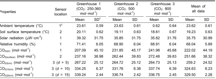
Table 1. Descriptive statistics of measured properties for the calibration period.

Properties Sensor

location

Greenhouse 1 (CO

: 250-360

mol･mol

)

Greenhouse 2 (CO

: 500 mol･mol

)

Greenhouse 3 (CO

: 800 mol･mol

)

Mean of all data

Mean SD

Mean SD Mean SD Mean SD

Ambient temperature (°C) 1

23.61 0.59 23.63 0.61 0.62 0.64 23.62 0.61

Soil surface temperature (°C) 2 20.11 0.62 19.11 0.63 18.61 0.67 19.23 0.63

Solar radiation (μW･cm

) 1 39.32 31.75 35.85 31.75 35.82 31.76 35.75 30.99

Relative humidity (%) 1 71.41 6.05 68.90 6.04 68.91 6.04 68.04 5.89

CO

(mol･mol

) 1 207.09 45.10 231.85 45.17 241.98 45.68 222.02 44.19

CO

(mol･mol

) 2 237.16 38.98 262.44 39.83 272.48 39.83 251.66 38.32

CO

(mol･mol

) 3 (d = 5) 267.22 25.12 264.72 25.12 264.73 25.13 259.2 24.52

CO

(mol･mol

) 3 (d = 10) 334.25 6.37 331.76 6.38 337.74 6.39 324.63 6.23

CO

(mol･mol

) 3 (d = 15) 339.24 2.44 336.74 2.42 336.75 2.45 329.50 2.28

z

SD: Standard deviation (n = 720).

y

Index of sensor location in Fig. 1.

Automacao Inc., USA) was used to measure relative humidity, and a NDIR (Non Dispersive Infra Red) sensor (KCD-1, Korea Digital Inc., Korea) was used for continuous monitoring of CO

concentration. The NDIR sensor was a simple spectro- scopic device often used to detect CO

molecules absorbing light at 4.26 μm. Range and resolution of the sensor were 0-2,000 μmol･mol

and 2 μmol･mol

, respectively. A micro- fluid pump was positioned between the NDIR sensor and a porous filter to transfer CO

gas from different soil depths (Fig. 1B). Through preliminary testing in a closed chamber, flow rate of the micro-fluid pump was set to 0.9 L･min

to maintain sufficient gas flow from the soil. Multiple filter- pump-sensor systems were employed to measure the CO

concentration at the different soil depths. The benefit of this method was the ability to measure the CO

concentration nondestructively and continuously after the apparatus was

installed at a particular soil depth.

Data were collected for 14 days for the development of empirical models estimating CO

levels using the environmental factors, and also for another 10 days for validation of the models. There was relatively less variance in temperature at the soil surface and CO

concentrations at certain soil depths (10 and 20 cm) during the calibration period (Fig.

2). CO

concentration was greater and the variances were

lower as the measurement depth was increased. Considering

the variance in CO

concentration, it could be recognized

that there might be some relationship between the change

of CO

in the soil and solar radiation in certain time periods

(i.e., from 6:00 to 8:00 and from 16:00 to 18:00). This

examination led us to conduct a closer investigation of

segmentation of predictor and response variables in shorter

time periods in regression analysis. Mean and standard deviation

Table 2. Models, variables, and variable transformations used in the regression analysis.

Type Model function Predictorvariable (x) Response variable (y)

LR y = β

Environmental variables Transformation CO

concentration at Ambient air, Surface of soil 5 cm depth of soil 10 cm depth of soil 20 cm depth of soil And their difference

RR y = βx + ε

Soil temperature Solar radiation Relative humidity

x

x 1 log (x)

e

P2 y = β

+ ε P3 y = β

+ β

+ ε

GN y = β(x)

+ ε

z

Coefficient.

y

Error term.

x

Inverse of the normal cumulative distribution function.

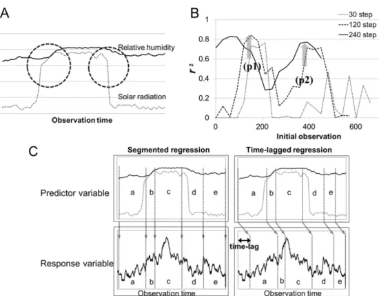
Fig. 3. Considerable variability found within the region of dotted circle in plots of solar radiation and relative humidity (A). Plots of coefficient of determination from regression analysis as a function of observation width and initial observation (B). An illustration of the time-lag between predictor and response variables in time-lagged regression (C).

of the measured environmental properties for each experimental greenhouse was shown in Table 1.

Analytical Procedures

To determine the relationships between CO

concentration vs. environmental properties, various regression models were tried: linear regression (LR), robust linear regression (RR), second order (quadratic) polynomial regression (P2), third order (cubic) polynomial regression (P3), and a generalized linear model using the inverse of the normal cumulative distribution function as the link function (GN). Preliminary analysis (Lee et al., 2011) showed that no significant regression models were found between the CO

concentration and environ-

mental variables such as soil temperature, solar radiation, and relative humidity. When using the difference between CO

concentrations at different soil depths as a response variable, however, relatively strong and significant relationships were obtained with solar radiation and relative humidity as predictor variables in some cases. Based on the preliminary analysis, a line arregression model as in equation 1 was introduced and multiple linear regression analysis was per- formed to determine the regression coefficients. Models were evaluated with original and transformed forms of solar radiation (W) and relative humidity (H) data (Table 2).

C

- C

= β

+ β

W + β

H + e (1)

Table 3. Coefficient of determination (r

) obtained with different transformations of predictor variables for the calibration dataset.

Predictor variable x

is solar radiation, predictor variable x

is relative humidity, and response variable y is CO

. Transformation of thepredictors

x

, x

x

1

, x

1

log (x

), log (x

) e

, x

x

, e

e

, e

0.7963 0.7378 0.7693 0.8031 0.7981 0.8044

Table 4. Results of multiple linear regression using optimized regression type and variable transformation for the calibration dataset.

Model ID Predictor variable x

= solar radiation Predictor variable x

= relative humidity

Response variable y = CO

r²

RMSEC β

β

β

1 x

, x

0.7963 5.08 0.1749 0.7410 -31.233

2 e

, x

0.8293 4.65 0.0217 0.3369 -2.0473

where,

Csurface : CO

concentration at soil surface, C

: CO

concentration at a 5-cm soil depth, W : original or transformed solar radiation, H : original or transformed relative humidity, β

, β

, β

: constant and regression coefficients, and e : error term.

During multiple linear regression analysis, calibration of the model was carried out in several ways. Through observation of the data (Fig. 3A), regression was applied for segmented sub-data sets of short time periods to obtain different regression coefficients for different portions of the whole data. Segmented regression (Berman et al., 1996; Cox, 1996; Shuai et al., 2003) is useful when the relationship between dependent and independent variables is different in these segments. The boundaries between the segments are called ‘breakpoints’. To determine the breakpoints, regression analysis was performed iteratively by varying the initial observation and observation width (Fig. 3B). By taking the maximum coefficient of determination indicated by p1 (Fig. 3B), the first segmented partition (from initial observation point to initial point plus observation width) was determined. For the second segmented partition, the next representative peak value (p2 in Fig. 3B) was selected. Another iterative time-lagged regression analysis (Körnet et al., 2007) was also used to develop a more practical model considering the time dependent nature of change in CO

emission from the soil affected by solar radiation and relative humidity. With this method, each observation in the response variable (CO

) is shifted by a time-lag per iteration step, after the determination of breakpoints (Fig. 3C).

Results and Discussion

First, the type of regression model and optimum transfor-

mation of the independent (predictor) variables were determined.

Different regression methods and transformations as listed in Table 2 were applied to the calibration dataset. Comparison of the results showed that the best coefficients of determination were obtained with linear regressions using original and exponential forms of predictor variables, as shown in bold in Table 3. Based on these results, linear regression was used for the remainder of the analysis.

The next step was to optimize the exponential transformation of the input predictors. Initial screening used a transformation of the form exp (x/100), but for final model development the optimum value of the constant was determined. Multiple linear regression (MLR) analysis runs were completed iteratively varying the constant, k, in exp (x/k) from 1 to 100. Exami- nation of the coefficient of determination across the range of k in the exponential formula for solar radiation showed that the transformation exp (x/12) was the best. Thus, the transformation exp (x/12) was used for solar radiation for the remainder of the analysis. Two candidate multiple linear regression models developed were summarized in Table 4.

Through iterative regression analysis, optimum segmented partitions of the measurements were determined for each greenhouse (Table 5). The whole data were partitioned into five segments, and the breakpoints determined were different for the different greenhouses. The two most important partitions were segments b and d, sub-data sets for after sun-rise and before sun-set, since these two breakpoint ranges gave the best coefficients of determination. For the calibration of the candidate models 1 and 2 using data from all of the green- houses, the breakpoints for the mean data from all greenhouses were selected.

The two candidate models were evaluated by the segmented and time-lagged regression analyses. While r

values were relatively low when MLR analysis was applied to the other segments, good fits were obtained for segments b and d.

Model 1 gave the best coefficient of determination for the

Table 5. Breakpoints from the segmented regression for datasets from each greenhouse and mean values of all greenhouses.

Segment ID

Greenhouse 1 (CO

: 250-360 mol･mol

)

Greenhouse 2 (CO

: 500 mol･mol

)

Greenhouse 3

(CO

: 800 mol･mol

) Mean of all data

Initial Width Initial Width Initial Width Initial Width

a 1

169 1 169 1 139 1 180

b 170 35 150 50 140 60 181 24

c 206 173 201 149 201 149 205 163

d 380 130 380 190 350 150 368 199

e 511 209 511 179 501 219 567 153

z

1 unit = 2 min.

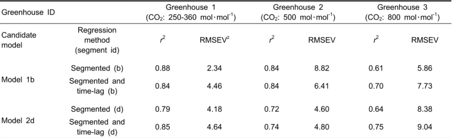
Table 6. Results of validation of each candidate regression model on the three experimental greenhouses.

Greenhouse ID Greenhouse 1

(CO

: 250-360 mol･mol

)

Greenhouse 2 (CO

: 500 mol･mol

)

Greenhouse 3 (CO

: 800 mol･mol

) Candidate

model

Regression method (segment id)

r²

RMSEV

RMSEV

RMSEV

Model 1b

Segmented (b) 0.88 2.34 0.84 8.82 0.61 5.86

Segmented and

time-lag (b) 0.84 4.46 0.84 6.41 0.70 7.73

Model 2d

Segmented (d) 0.79 4.18 0.72 4.60 0.64 8.38

Segmented and

time-lag (d) 0.85 4.64 0.74 4.80 0.75 9.04

z

RMSEV: Root mean square error of validation.

b segment, measurements from 6:02 to 6:50 AM (from 181 to 181 + 24 in Table 5), model 2 performed well in the d segments, measurements of 12:16 to 6:54 PM (from 368 to 368 + 199 in Table 5). Model 1 with the b segment (indicated by Model 1b) and the d segment (indicated by Model 1d) gave coefficient of determination of r

= 0.93 and r

= 0.85, respectively. Model 2 with the b segment (indicated by Model 2b) and the d segment (indicated by Model 2d) both gave coefficients of determination of r

= 0.87. The two models showed the same optimum time lag (8 min or 4 measurements) in the b segment but different lags in the d segment (0 and 10 min). These results suggested that the model could estimate the response values better with the determined time-lag.

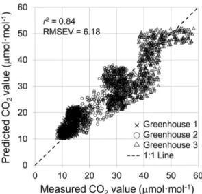
The four models were evaluated with the validation datasets from three experimental greenhouses with using the defined segments and time-lags. Two models showed relatively high coefficients of determination throughout all greenhouses (Table 6). Model 1b gave greater coefficients of determination in the b segment (Table 5) of all the greenhouses, while model 2d gave greater coefficients of determination in the d segment (Table 5) of all the greenhouses. The models showed relatively high correlation in the different segments regardless of the type of CO

enrichment, the correlation between the concentration

of CO

and the solar radiation, but greenhouses with greaterCO

enrichment setting resulted in a greater root mean square error of validation (RMSEV) for most of the models.

Based on these results, we suggested two empirical models to estimate the difference of CO

concentrations at different depths. Equation 2 is one part of the suggested empirical model to estimate the concentration of CO

between observations 182 and 205 (between 6:02 and 6:50 AM) with an 8-min time-lag Equation 3 represents the other partition between observations 368 and 567 (between the time range of 12:16 and 6:54 PM) with a 10-minute time-lag.

(C

- C

)

= 0.9618W

+ 0.4502H

- 28.464 (2) (C

- C

)

= 0.0217e

Wt

12

- 0.1238H

+ 30.373 (3)

where,

C : CO

concentration at a soil depth, t : observation time in minutes, W

: solar radiation at time t, H

: relative humidity at time t.

Using the validation dataset, the concentration of CO

was predicted by the empirical models as described by Equation

Fig. 4. Scatter plot of measured and predicted CO

values for the validation dataset.

2 and 3. The coefficients of determination for each greenhouse were not strongly high, but the empirical model was somewhat more robust against the different CO

enrichment methods considering the overall coefficient of determination was 0.84 (Fig. 4).

In this study, a mathematical model was developed to relate key environmental factors to CO

concentrations measured at different depths. Predictor variables selected were original and exponential transformation of solar radiation and relative humidity. The difference of CO

concentrations between the surface and 5-cm soil depth was chosen as the response variable. The models were applied to segmented sub-datasets of shorter time periods, and better models were obtained for measurements at “after sun-rise” and “before sun-set”

periods when there was more variability in solar radiation and relative humidity than in other time frames. To consider time delay in the response of CO

concentration, time-lagged regression analysis was used. As a result, there was an improvement in coefficients of determination (0.93 and 0.87) with the segmented time frames. The developed model resulted in an overall coefficient of determination of 0.84 forthe 10-day validation dataset.

Literature Cited

Berman, N.G., W.K. Wong, S. Bhasin, and E. Ipp. 1996. Application of segmented regression models for biomedical studies. Am.

J. Physiology 270:723-732.

Caetano, M.A.L., D.F.M. Gherardi, and T. Yoneyama. 2008.

Optimal resource management control for CO

emission and reduction of the greenhouse effect. Ecol. Model. 213:119-126.

Camarda, M., S. Gurrieri, and M. Valenza. 2009. Effects of soil gas permeability and recirculation flux on soil CO

flux measurements performed using a closed dynamic accumulation

chamber. Chem. Geol. 265:387-393.

Chen, F. and Y. Tang. 2010. Towards constraint optimal control of greenhouse climate. In Proc. LSMS/ICSEE p. 439-450.

Cox, F.R. 1996. Economic phosphorus fertilization using a linear response and plateau function. Commun. Soil Sci. Plan. 27:

531-543.

DeSutter, T.M., T.J. Sauer, and T.B. Parkin. 2006. Porous tubing for use in monitoring soil CO

concentrations. Soil Biol.

Biochem. 38:2676-2681.

Fang, C. and J.B. Moncrieff. 1999. A model for soil CO

pro- duction and transport 1: Model development. Agr. Forest Meteorol. 95:225-236.

Filipovic, D., S. Kosutic, Z. Gospodaric, R. Zimmer, and D. Banaj.

2006. The possibilities of fuel savings and the reduction of CO

emissions in the soil tillage in Croatia. Agr. Echosyst.

Environ. 115:290-294.

Granieri, D., G. Chiodini, W. Marzocchi, and R. Avino. 2003.

Continuous monitoring of CO

soil diffuse degassing at Phlegraean fields (Italy): Influence of environmental and volcanic parameters. Earth Planet Sc. Lett. 212:167-179.

Jassal, R.S., T.A. Black, G.B. Drewitt, M.D. Novak, D. Gaumont- Guay, and Z. Nesic. 2004. A model of the production and transport of CO

in soil: Predicting soil CO

concentrations and CO

efflux from a forest floor. Agr. Echosyst. Environ.

124:219-236.

Jeong, C.S, J.N. Park, and J.H. Kyoung. 2006. Effect of high CO

short-term treatment on the respiration characteristics and quality of broccoli. Kor. J. Hort. Sci. Technol. 24:447-451.

Kabwe, L.K., M.J. Hendry, G.W. Wilson, and J.R. Lawrence.

2002. Quantifying CO

fluxes from soil surfaces to the atmosphere.

J. Hydrol. 260:1-14.

Körnet, O., A.V. Ooster, and M. Hulsbos. 2007. Design and performance of a measuring system for CO

exchange of a greenhouse crop at different light levels. Biosyst. Eng. 97:

219-228.

Lee, D.H., K.S. Lee, C.H. Choi, H.J. Kim, S.O. Chung, and Y.J.

Cho. 2011. Prediction of CO

emission from soil for optimal greenhouse control. Proc. Amer. Soc. Agr. Biol. Eng. No.

1111628.

Li, Y.-L., D. Otieno, K. Owen, Y. Zhang, J. Tenhunen, X.-Q.

Rao, and Y.-B. Lin. 2008. Temporal variability in soil CO

emission in an orchard forest ecosystem. Pedosphere 18:

273-283.

Lou, Y., Z. Li, T. Zhang, and Y. Liang. 2004. CO

emissions from subtropical arable soils of China. Soil Biol. Biochem.

36:1835-1842.

Maestre, F.T. and J. Cortina. 2003. Small-scale spatial variation in soil CO

efflux in a Mediterranean semiarid steppe. Appl.

Soil Ecol. 23:199-209.

Ouyang, Y. and C. Zheng. 2000. Surficial processes and CO

flux in soil ecosystem. J. Hydrol. 234:54-70.

Park, S.A, M.G. Kim, M.H. Yoo, M.M. Oh, and K.C. Son. 2010.

Comparison of indoor CO

removal capability of five foliage plants by photosynthesis. Kor. J. Hort. Sci. Technol. 28:

864-870.

Pohlheim, H. and A. Heiβnet. 1999. Optimal control of greenhouse climate using real-world weather data end evolutionary algorithms.

Proc. Genetic Evolutionary Computation Conf. 1672-1677.

Shuai, X., Z. Zhou, and R.S. Yost. 2003. Using segmented regression models to fit soil nutrient and soybean grain yield changes due to liming. J. Agric. Biol. Environ. Stat. 8:240-252.

Smart, D.R. and P. Josep. 2005. Short-term CO

emissions from planted soil subject to elevated CO

and simulated precipitation.

Appl. Soil Ecol. 28:247-257.

Subke, J.A., R. Markus, and D.T. John. 2003. Explaining temporal variation in soil CO

efflux in a mature spruce forest in Southern Germany. Soil Biol. Biochem. 35:1467-1483.

Takahashi, A., T. Hiyama, H.A. Takahashic, and Y. Fukushima.

2004. Analytical estimation of the vertical distribution of CO

production within soil: Application to a Japanese temperate forest. Agr. Forest Meteorol. 126:223-235.

Tang, J., D.D. Baldocchi, Y. Qi, and L. Xu. 2003. Assessing soil CO

efflux using continuous measurements of CO

profiles in soils with small solid-state sensors. Agr. Forest Meteorol. 118:207-220.

Zhang, H., W. Xiaoke, F. Zongwei, S. Wenzhi, L. Wenzhao, and O. Zhiyun. 2007. Multichannel automated chamber system for continuous monitoring of CO

exchange between the agro-ecosystem or soil and the atmosphere. Acta Ecol. Sin.

27:1273-1282.