1. Introduction
Suspended sediment is an important index for monitoring changes in coastal environment. The coastal area has exhibited great fluctuation of Suspended Sediment Concentration (SSC) to exert a critical influence on local ocean condition once in a
while. The suspended sediment may be originated from various sources such as re-suspension of bottom deposit, river-borne particles, eroded matter from coastal area, sediment of dredge, and so on. It shows higher level of concentration at the coastal area than open ocean (Gordon, 1983).
Spectral characteristics of sea water are mainly
Estimation of Coastal Suspended Sediment Concentration using Satellite Data and Oceanic In-Situ Measurements
Min-Sun Lee*, Kyung-Ae Park**, ***†, Jong-Yul Chung***, Yu-Hwan Ahn**** and Jeong-Eun Moon****
*Department of Science Education, Seoul National University
**Department of Earth Science Education, Seoul National University
***Research Institute of Oceanography, Seoul National University
****Korea Ocean Research and Development Institute
Abstract : Suspended sediment is an important oceanic variable for monitoring changes in coastal environment related to physical and biogeochemical processes. In order to estimate suspended sediment concentration (SSC) from satellite data, we derived SSC coefficients by fitting satellite remote sensing reflectances to in-situ suspended sediment measurements. To collect in-situ suspended sediment, we conducted ship cruises at 16 different locations three times for the periods of Sep.-November 2009 and Jul.
2010 at the passing time of Landsat ETM+. Satellite data and in-situ data measured by spectroradiometers were converted to remote sensing reflectances (Rrs). Statistical approaches proved that the exponential formula using a single band of Rrs(565) was the most appropriate equation for the estimation of SSC in this study. Satellite suspended sediment using the newly-derived coefficients showed a good agreement with in- situ suspended sediment with an Root Mean Square (RMS) error of 1-3 g/m3. Satellite-observed SSCs tended to be overestimated at shallow depths due to bottom reflection presumably. This implies that the satellite-based SSCs should be carefully understood at the shallow coastal regions. Nevertheless, the satellite- derived SSCs based on the derived SSC coefficients, for the most cases, reasonably coincided with the pattern of in-situ suspended sediment measurements in the study region.
Key Words :Suspended Sediment, Landsat ETM+, Remote Sensing Reflectance
Received November 4, 2011; Revised November 28, 2011, Revised December 19, 2011; Accepted December 20, 2011.
†Corresponding Author: Kyung-Ae Park ([email protected])
related to ocean color with diverse sources, especially the concentration of suspended sediments over relatively shallow depth in coastal region. In general, the spectral reflectance of sediment-dominated water shows increasing absorption at both the red and blue wavelengths in the electromagnetic spectrum and U- shaped feature at green wavelength (Sathyendranath and Morel, 1983). Suspended sediment as inorganic matter is an excellent scattering material without any absorption of solar radiance. Magnitude of the scattering is related to the size of each sediment and its distribution. As the sediment becomes small, so the capacity for scattering gets large. Since the previous literature based on empirical models has reported that specific kinds of sediments were related to water leaving radiances at specific spectral wavelength (Robinson, 2004).
Monitoring of suspended sediment concentration using in-situ measurement is limited spatiotemporally, whereas, satellite remote sensing has offered a chance to overcome the limits by its spatial distributions. The suspended sediment dominantly reflects at wavelength of 500-600 nm, thus, it may be possible to determine the concentration of suspended sediment using these wavelengths. Clark (1980) utilized the ratio of spectral radiance at 440 nm and 550 nm of Coastal Zone Color Scanner (CZCS) for Nimbus pre- launch research in order to estimate suspended sediment. Other studies estimated suspended sediment using satellite data (e.g., Clark, 1980;
Strum, 1983; Tassan, 1994; Clark, 1997; Doerffer and Schiller, 1997; Binding, 2003; Ruddick, 2003;
Miller and McKee, 2004).
Since the coastal region around Korea has relatively shallow depths, its coastal environment is liable to contain bunch of suspended sediments.
Some of the previous researches performed to develop the algorithm of suspended sediments in Lake Sihwa and coastal area (Jeong et al., 1999;
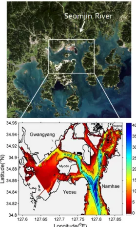
Jeong, 2001) and in Saemangeum area (Min et al., 2006). We selected Gwangyang Bay as one of the potential areas with large suspended sediments in the southern coast of Korea. The bay is 17 kilometers long and 9 kilometers across with relatively shallow depth of less than 40 m as shown in Fig. 1. The sediment in the bay were reported to be mainly originated from the suspended matter from the Seomjin river at adjacent estuary northward and from sedimentary layer in the west coast of the Gwangyang Bay and Yeosu Bay (Kim and Kang, 1991). Tidal range is about 3 m and the ratio of seawater exchange by tides amounts to 7.6-22.3%
which is greatly changed by riverine inflow (Park et al., 1984). In addition, there are lots of sources of the suspended sediment generated by human activities
Fig. 1. Bottom topography (m) of the study region.
like dredge, quay construction, farming and fisheries, and so on. Therefore, various causes have been anticipated to affect spatial distribution and concentration of suspended sediment in the Gwangyang Bay.
The objectives of this study are (1) to understand the relationship between spectral characteristics of suspended sediment by on-board experiment with spectroradiometer and in-situ measurements of suspended sediment by filtering works, (2) to retrieve empirical coefficient to estimate concentration of suspended sediment from satellite data, and (3) to discuss potential errors in the interpretation of SSC image from satellite data.
2. Data
1) Satellite Data
In order to obtain SSC, satellite sensor should observe radiance from the surface at several visible bands. There are some representative satellites to meet the requirements for ocean color monitoring such as Moderate Resolution Imaging Spectroradiometer (MODIS), Sea-viewing Wide Field-of-view Sensor (SeaWiFS), Medium Resolution Imaging Spectrometer (MERIS), and so on. However, these satellite data have relatively low spatial resolution of about 1 km, which is somewhat inappropriate for the small study region with a length of 17 km. Other satellites such as Korea Multi-Purpose Satellite-2 (KOMPSAT-2) or IKONOS with much higher spatial resolutions to cover the study region, however those were unavailable during the study period. Thus, we selected Landsat ETM+ in spite of the well-known problem with striped patterns due to its sensor malfunction (Parkinson, 2006).
The Landsat ETM+ has observed the research area
with 16-day revisit period and 30-m spatial. The wavelength and spatial resolution of the Landsast ETM+ are summarized in Table 1. It includes visible wavelengths (blue, green, and red), near infrared, and thermal infrared wavelengths. The green and red wavelengths centered at 565 nm and 660 nm may be useful for estimating suspended sediment. The Landsat ETM+ scanned 24 times over the study region during the present research period from May 2009 to Aug. 2010. Only 15 scenes of the 24 observations, however, could be used because of clouds or partly clouds. We obtained the Landsat ETM+ data from USGS (U.S. Geological Survey) website.
2) In-Situ Data
We conducted shipboard in-situ observations for days forecasted clear weather condition from May 2009 to Aug. 2010. Table 2 shows the details of the cruises. The cruises were conducted three times on 22 Sep. 2009, 25 Nov. 2009, and 7 Jul. 2010 during the satellite overpasses over the study region. Total duration of each ship cruise took a few hours from 9 h to 13 h approximately. Although the weather forecast reported clear condition, it frequently did not coincide with actual weathers as our first cruise on 22 Sep. 2009. However, during this period, we also collected a good quality of in-situ measurements.
Fortunately, the second and the third cruises were Table 1. Spectral characteristics of Landsat ETM+ and resolutions No. Band Range (mm) Band Resolution (m)
1 0.450-0.515 Blue 30
2 0.525-0.605 Green 30
3 0.630-0.690 Red 30
4 0.760-0.900 Near IR 30
5 1.550-1.750 Mid IR 30
6 10.40-12.5 Thermal 60
7 2.080-2.35 Mid IR 30
8 0.52-0.92 Pan 15
No. Band Range (mm) Band Resolution (m)
conducted under clear conditions and could obtain satellite images. However, the different instruments were inevitably used such as dual spectroradiometer during the second campaign and single spectroradiometer during the third campaign, respectively. Fig. 2 illustrates the locations of observation stations which were subjectively selected to include a wide range of suspended sediment concentration values according to a priori results from our previous field surveys. The numbers of each stations in colored circles represent the order of the measurements during the first cruise (Fig. 2).
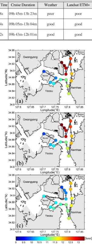
Fig. 3 shows the stations with arrows which denote the order and moving directions of the measurements of water sampling. If suspended sediment varies with time, the orders may affect on the errors of satellite suspended sediment estimation because of
Table 2. Information of three cruises and satellite overpasses
No. Date Instrument Satellite Passing Time Cruise Duration Weather Landsat ETM+
1 22 Sep. 2009 ASD dual
10h 55m 48s 09h 45m-13h 23m poor poor
spectroradiometer
2 25 Nov. 2009 ASD dual
10h 56m 24s 09h 05m-13h 04m good good
spectroradiometer
3 7 Jul. 2010 ASD single
10h 57m 52s 09h 43m-12h 01m good good
spectroradiometer
No. Date Instrument Satellite Passing Time Cruise Duration Weather Landsat ETM+
Fig. 2. The RGB composite image of Landsat ETM+ data in the study region on 16 Sep. 2001, where the numbers in colored circles represent the station numbers from 1 to 16.
Fig. 3. The ship tracks conducted on (a) 22 Sep. 2009, (b) 25 Nov. 2009, and (c) 7 Jul. 2010, where the arrows indicate the direction of ship movement and colors represent the order of the stations of each day.
considerable time intervals between the water sampling and satellite observation. It was used to decide whether SSC errors were caused by the time difference between satellite scanning time and in-situ observation or not and to understand the potential sources of the SSC errors.
3. Method
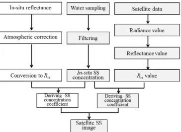
The research procedure was made up of the processing of in-situ measurements, satellite data processing and conversions, and calculating SSC coefficients to derive suspended sediment from satellite data based on in-situ measurements of SS.
Fig. 4 presents the flowchart of the research. The left- side column describes the conversion procedure of in- situ remote sensing reflectance. The middle one shows the steps of in-situ SSC from water sampling.
The right-side illustrates the conversion of satellite data into the remote sensing reflectance to be used in deriving SSC coefficients for satellite remote sensing reflectance data. Satellite SSCs were calculated by applying the retrieved coefficients to satellite remote
sensing reflectances. The shaded portion represents the main procedure of this study. Detail procedures are in the following.
1) Filtering of Sea Water
Satellite data should be validated with in-situ measurements. The accuracies of the satellite-derived variables depend on the accuracy of the oceanic measurements conducted on shipboard using precise instruments. During the campaigns performed at similar time with an hour as compared with satellite overpassing time on the same date, we sampled 1-liter of waters near the sea surface at every stations using Niskin sampler. The sampled water was filtered by GF/C (glass filter type C) and generated suspended sediment concentration data in the unit of g/m3. 2) Filling Striped Patterns
The scan line corrector of the Landsat ETM+ was out of order on 31 May 2003. It had long played an important role in preventing the ‘zig-zag’ motion during the along and across track motion. After the scan line corrector was failed, 22% of Landsat ETM+
images have not been scanned properly by increasing
Fig. 4. A flow chart of data processing procedures related to in-situ measurements, data processing and conversion, and calculating suspended sediment concentration coefficients to retrieve satellite-observed SS.
the gaps from the center to the edge of a scene (Parkinson, 2006). However, the scanned portion was known to have no problems to be used in diverse applications. It does not have other serious problems except for the stripes, so that we decided to use the scanned image for the study by developing the removal technique of the patterns. Since the Landsat ETM+ data have been widely used, various researches have exerted to restore the images (Chen, 2011). Most of the studies were mainly performed for land applications by the comparison of the erroneous image with the past image without any problem.
However, these might not be useful for oceanic applications because ocean changes more rapidly than land and also because ocean colors vary at a narrow range of reflectances. Thus, we utilized a fundamental filling method that interpolated the values of neighborhood pixels to the un-scanned pixels with 7×7 moving averages. The kernel size was determined by considering the width of striped patterns, 4-6 pixels in this study.
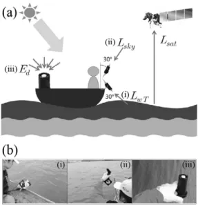
3) Conversion of In-Situ Measurement The optical properties such as total water leaving radiance (LwT, W/m2/nm/sr), sky radiance(Lsky, W/m2/nm/sr), and down-welling irradiance (Ed, W/m2/nm) were measured on the shipboard.
Schematic concept of the in-situ measurement during the satellite passing was illustrated in Fig. 5. The sky radiance Lsky was measured by pointing the sky upward by 30˚ under clear sky condition and the LwT was measured by the same angle with Lsky((i) and (ii) in Fig. 5b). The Ed for the hemisphere incoming to the sea surface was measured by Remote Cosine Receptor (RCR) of ASD as shown in (iii) of Fig. 5b.
The remote sensing reflectance was defined as:
Rrs= = , (1)
where Fris Fresnel reflection coefficient at the water surface, Lwis water leaving radiance (W/m2/nm/sr) and calculated by measured LwT, Lsky, and Ed. These optical data were measured with 1-nm spectral resolution using spectroradiometer. Measured LwT included skylight reflection effects, therefore, it was corrected by measured sky radiance Lsky and Fr (Mobley, 1999). The several values of Fr has suggested by the previous studies (Ball, 1954; Austin, 1974; Ahn, 1990). In this study, Frvalue was selected to 0.025 as a proper value in the coastal region of Korea (Ahn, 1990). Finally, the converted Rrswas multiplied by the response functions of each ETM+
band.
4) Conversion of Satellite Data
The remote sensing reflectance Rrswas defined as:
Ll= (Qcal_ Qcalmin) + LMINl (2),
rl= (3),p×(Ll_ Ldp)×d2 ESUN×cos(90˚ _ q)×p/180˚)×t LMAXl_ LMINl
Qcalmax_ Qcalmin
LwT_ (Lsky ×Fr) Ed Lw
Ed
Fig. 5. (a) Schematic diagram of on-board measurement procedures for LwT(total water leaving radiance), Lsky
(sky radiance), Ed (down-welling irradiance), and Lsat
(satellite observing radiance), where (i), (ii), and (iii) of (b) are the photos to measure LwT, Lsky, and Ed, respectively.
Rrsl= , (4) where Llis spectral radiance at the sensor’s aperture
(W/m2/mm/sr), Qcalis quantized calibrated pixel value range from 0 to 255, Qcalminis minimum quantized calibrated pixel value 0 corresponding to LMINl, Qcalmaxis maximum quantized calibrated pixel value 255 corresponding to LMAXl, LMINl is minimum spectral at-sensor radiances that are scaled to Qcalmin (W/m2/mm/sr), LMAXl is maximum spectral at- sensor radiances that are scaled to Qcalmax(W/m2/ mm/sr), rlis water surface reflectance (unitless), Ldp is atmospheric correction term (Chavez, 1996) and the value converted the dark pixel into Ll, d is distance between Earth and Sun (astronomical units), ESUN is mean atmospheric solar irradiance rl
p
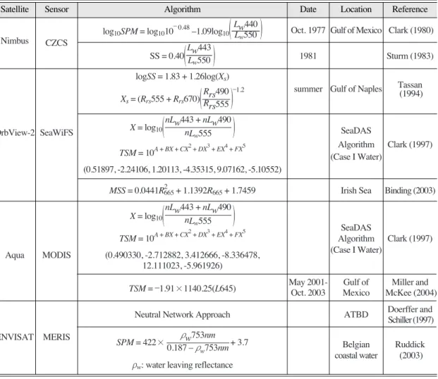
Table 3. Summary of the equations for suspended sediment concentration retrievals from satellite in the previous studies
Satellite Sensor Algorithm Date Location Reference
Nimbus CZCS
log10SPM = log1010
_ 0.48_1.09log10
( )
Oct. 1977 Gulf of Mexico Clark (1980)SS = 0.40
( )
1981 Sturm (1983)logSS = 1.83 + 1.26log(Xs)
summer Gulf of Naples Tassan
Xs= (Rrs555 + Rrs670)
( )
_1.2 (1994)OrbView-2 SeaWiFS X = log10
( )
SeaDASTSM = 10A + BX + CX2+ DX3+ EX4+ FX5 Algorithm Clark (1997) (0.51897, -2.24106, 1.20113, -4.35315, 9.07162, -5.10552)
(Case I Water)
MSS = 0.0441R2665+ 1.1392R665+ 1.7459 Irish Sea Binding (2003)
X = log10
( )
SeaDAS TSM = 10A + BX + CX2+ DX3+ EX4+ FX5
Algorithm Clark (1997) Aqua MODIS (0.490330, -2.712882, 3.412666, -8.336478, (Case I Water)
12.111023, -5.961926)
TSM = _1.91×1140.25(L645) May 2001- Gulf of Miller and Oct. 2003 Mexico McKee (2004)
Neutral Network Approach ATBD Doerffer and
Schiller (1997) ENVISAT MERIS
SPM = 422× + 3.7 Belgian Ruddick
rw: water leaving reflectance
coastal water (2003)
Satellite Sensor Algorithm Date Location Reference
Lw443 Lw550
Rrs490 Rrs555 nLw443 + nLw490
nLw555
nLw443 + nLw490 nLw555
rw753nm 0.187 _ rw753nm
Table 4. Equation forms for the estimation of suspended sediment concentrations, where Rrsis satellite remote sensing reflectance and the numbers (485, 555, 565) represent the central wavelengths of the bands of satellite sensor with a unit of nm
Type Equation
R1 SS = c1ec2Rrs(565) R2 SS = c1Rrs(565) + c2
R3 SS = c1ec2Rrs(485)/Rrs(565) R4 SS = c1Rrs(485)/Rrs(565) + c2
Type Equation
Lw440 Lw550
(W/m2/nm), q is solar zenith angle (degrees), t is atmospheric penetration rate and applied by cosq (Chavez, 1996), and Rrsis remote sensing reflectance.
Ldp was selected a value at the darkest pixel throughout the entire image.
The reflectance (rl) in (3) was converted to Rrs
from the equation (4).
5) Retrieval of SSC Coefficient
Several researches to retrieve SSC from satellite data have been performed to determine the proper SSC estimation equation and coefficients as summarized in Table 3. For example, many of ocean color satellite data from Nimbus/CZCS, OrbView- 2/SeaWiFS, Aqua/MODIS, and ENVISAT/MERIS have been used for the retrieval of SSC. In the most cases, the studies were focused on the open ocean with relatively large scale like as the Gulf of Mexico, the Gulf of Naples, the Irish Sea, and the Belgian coast.
The algorithms in Table 3 have used several wavelengths centered at 440, 443, 490, 550, 555, 666, and 753 nm. Landsat ETM+ does not contain the specific bands for SSC and atmospheric corrections.
Therefore in-situ Rrswas used to decide which type of function was proper to estimate SSC. The previous algorithms may be divided into 4 categories according to the number of wavelength bands and the forms of SSC equations as exponential or least squared approach (Clark, 1980; Strum, 1983; Tassan, 1994; Clark, 1997; Doerffer and Schiller, 1997;
Binding, 2003; Ruddick, 2003; Miller and McKee, 2004). Table 4 shows the 4 categories with characteristic forms from R1 to R4, where we used two wavelengths (485 nm and 565 nm) available from Landsat data. The R1 and the R2 equations were exponential equations and least squared equation of 565 nm centered wavelength Rrs, respectively. The R1 and the R3 were based on
exponential relationship between suspended sediment and satellite remote sensing reflectance. By contrast, the R2 type utilizes the linear least squared equation to Rrs. The R4 type shows the linear least squared relationship between suspended sediment and remote sensing reflectance ratio of Rrs(485)/Rrs(565).
In order to select one form out of the algorithms, we assessed the accuracies for each types by regressing in-situ reflectances to in-situ SSC measurements. The selected form was used to calculate SSC from satellite data as shown in the third column in Fig. 4.
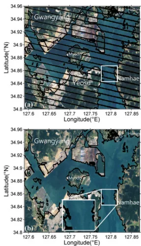
Fig. 6. Landsat RGB composite image (a) with stripes and (b) without stripes over the study region taken on 19 Sep.
2008, where the bigger white box indicates the enlarged image of the smaller white one.
4. Results
1) Filling of Stripes
Fig. 6a shows Landsat ETM+ RGB composite image with stripes taken on 19 Sep. 2008. As the filling procedure, the restored image in Fig. 6b looked clear without any stripes and showed the smooth variations of oceanic features without dominant discontinuity. The filled portion might have errors from the interpolation, but the overall feature seemed proper to perform the purpose of this study.
Fortunately, there was no station at which we conducted a cruise to collect in-situ measurement of SSC.
2) Spectral Characteristics of Suspended Sediment
In order to determine one of the ETM+ bands in the estimation of SSC coefficients, we had experiments with spectral measurements to confirm which wavelength range would be the most sensitive to SSC in sea waters. Fig. 7 shows in-situ spectral remote sensing reflectances using spectroradiometer as a function of wavelength. Among 16 stations, we arbitrarily selected 2 stations (7 and 15) with relatively large SSCs. The curves of spectral remote sensing reflectance showed large variations from 0.002 to 0.02 sr-1. The curves of the two stations showed quite a similar pattern in terms of the overall variations and the spectral peak around 565 nm. This supports the fact that sea water with large suspended sediment tends to have a spectral peak at 565 nm.
Landsat ETM+ has a band of which the central wavelength is 565 nm. Thus, we selected a band 2 center at 565 nm among other bands of Landsat ETM+. This band 2 data were consecutively utilized for the derivation of SSC coefficients for satellite data (Robinson, 2004).
3) Determination of SSC Algorithm
The survey of the previous literature revealed the 4 representative formulas for the estimation of SSC as shown in Table 4. Out of the algorithms, we should select one for the derivation of SSC retrievals. First of all, we performed the analysis of the first and the second columns on Fig. 4 by using in-situ Rrsand in- situ SSC. On the base of the RMS errors from regressions for the 4 types, the best algorithm was selected to be used next step.
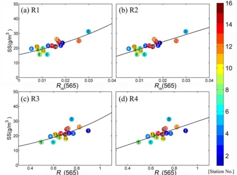
Fig. 8 presents the relationship between in-situ SSC and in-situ Rrsmeasured on Jul. 7, 2010. The concentration of in-situ suspended sediment had variations from 15.7 g/m3to 32.2 g/m3with an Fig. 7. (a) Remote sensing reflectances at stations 7 and 15
from in-situ data on 7 Jul. 2010 by using spectroradiometer and (b) difference of remote sensing reflectances between the two stations.
average value of 25.71 g/m3. The Rrs(565) measurements varied from 0.0054 to 0.0299 sr-1. Fig. 8a showed the exponential fitting between Rrs(565) and SS. The two variables showed relatively good agreement as compared with other approaches of R3 or R4. The R2 is a linearly least squared fit between the two as same with R1. The RMS errors of R1 and R2 were 2.2192 g/m3and 2.2710 g/m3, respectively (Table 5). From the small error of R1, the approach using the exponential relationship seemed to be better than the linear relationship of R2 in the case of Rrs(565).
When we measured Rrsat two bands of 485 nm and 565 nm, the values of Rrs(485) were lower than the values of Rrs(565) at the cruise stations. Therefore the ratios of the two bands, Rrs(485)/Rrs(565), were calculated to 0.4944-0.8984 as shown in Fig. 8c and d. RMS errors of R3 and R4 were 3.0051 g/m3and 2.9335 g/m3(Table 5). This implies that the linear relationship of R3 was better than the exponential relationship of R4 in the case of the ratio Rrs(485)/
Rrs(565). Therefore, the R1 type with exponential approach between a single band of Rrs(565) and in- situ suspended sediment was determined to the best equation. Thus, the R1 formula was utilized to derive SSC coefficients from satellite data. Each coefficients and the RMS errors for the types were summarized in Table 5.
In order to confirm whether the R1 formula was proper to the satellite Rrs, we compared in-situ Rrs with two images of satellite Rrson 25 Nov. 2009 and Fig. 8. Relationship between in-situ suspended sediment concentration and in-situ Rrsmeasured on 7 Jul. 2010 for the cases of (a) Rrs(565) with an exponential regression of R1, (b) Rrs(565) with a linear regression of R2, (c) ratio of Rrs(485) to Rrs(565) of R3 with an exponential regression, and (d) ratio of Rrs(485) to Rrs(565) with a linear regression of R4, where the colored numbers are the station numbers in Fig. 2.
Table 5. Statistical performances of suspended sediment algorithms by in-situ Rrs
Coefficients
c1 c2 RMSE (g/m3) Types
R1 15.5562 21.4729 2.2192
R2 492.7661 14.4204 2.2710
R3 8.8048 1.2745 3.0051
R4 26.7513 3.0828 2.9335
Coefficients
c1 c2 RMSE (g/m3) Types
7 Jul. 2010, where as the satellite image on 22 Sep.
2009 was not used because of cloudy condition over the research area (Fig. 9). The satellite Rrsare higher by 0.005 than in-situ Rrs(Fig. 9a), which might be induced by the effect of weak haze prior to stratocumulus approaching from the west. Moreover, the satellite distributed at the very narrow range of in- situ Rrs. In order to enhance the stability of the regression equation, the range of in-situ measurements should vary at a large range as possible. The other observations as shown in Fig. 9b satisfied the
condition of a large range of in-situ Rrs. Most of the satellite and in-situ measurement showed a good agreement with a relatively large range for regression.
Thus, we selected the satellite Rrson 7 Jul. 2010 for the calculation of SSC coefficients.
4) SSC Coefficient
In order to derive SSC coefficients for satellite data, we applied the procedures of the second and the third columns on Fig. 4. Fig. 10 shows the regressed line between in-situ SSC measurements and satellite Rrs(565) data on 7 Jul. 2010 based on the exponential approach of R1. The stations of 11 and 12 were contaminated by clouds on Landsat RGB composite image, hence the values of them were removed from the derivation of the coefficients. The Rrs(565) value at the station 16 was also removed due to strong bottom reflection caused by quay construction nearby. The satellite Rrs(565) varied from 0.0067 to 0.0256 sr-1. The retrieved exponential equation by using in-situ SSC measurements and satellite Rrs(565) data was as following
SS = 16.2064e15.3529Rrs(565) (5) where Rrs(565) is satellite remote sensing reflectance Fig. 10. Suspended sediment concentrations (g/m3) as a function of satellite Rrs(565), where the colored numbers represent the station numbers from the cruise observation.
Fig. 9. Comparison of satellite Rrswith in-situ Rrsobserved on (a) 25 Nov. 2009, and (b) 7 Jul. 2010.
at a central wavelength of 565 nm. RMS error of (5) was estimated to 3.9981 g/m3.
We compared the estimated values and in-situ SSC values as shown in Fig. 11. The satellite-derived SSC showed a good agreement with in-situ suspended sediment concentration with an RMS error of 3.9981 g/m3. The concentration of the station 16 seemed to be significantly deviated from the general trend. The value was estimated to about 32 g/m3, which was higher by 10 g/m3than the corresponding in-situ value of about 22 g/m3. This might be originated from the large value of satellite Rrs(565) induced by strong bottom reflection.
When we estimated suspended sediment from the satellite data by using the equation of the previous literature (e.g. Min et al., 2006), suspended sediment was extremely overestimated about 2 or 3 times as large as in-situ suspended sediment measurements.
Thus, regional optimization should be required to improve the accuracy of suspended sediment from satellite data.
5) Application of the SSC Equation to Satellite Image
Using the suspended sediment concentration coefficients derived from the satellite Rrs, satellite suspended sediment concentrations were calculated as illustrated in Fig. 12a. Pixels determined as land or clouds by near-infrared channel of Landsat ETM+
were masked in white color on satellite suspended sediment image of Fig. 12a. The satellite-derived SSC values varied from 10 g/m3to 32 g/m3, which is Fig. 11. Comparison of satellite-derived suspended sediment
concentration (g/m3) and in-situ suspended sediment concentration (g/m3), where the colored numbers represent the station numbers during the ship cruise.
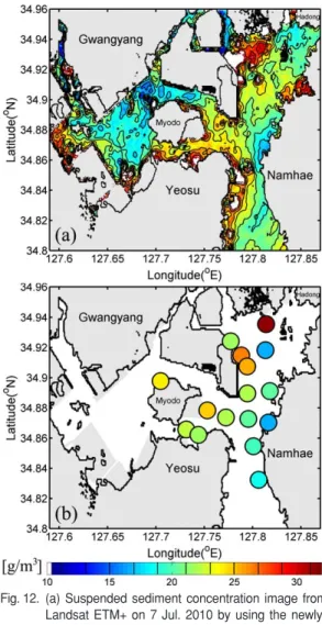
Fig. 12. (a) Suspended sediment concentration image from Landsat ETM+ on 7 Jul. 2010 by using the newly- derived SSC coefficients and (b) in-situ suspended sediment concentrations at each stations on the same day with satellite observation.
quite similar to the range of in-situ suspended sediment concentration values. High concentration of suspended sediment appeared at the estuary of the Seomjin River at 127.84˚E, 34.96˚N in the northern end of study region and along the coast of Yeosu. In overall, shallow coasts near land showed relatively large SSC. By contrast, clear ocean with less SSC was found along the deep channel between Namhae and Yeosu.
The in-situ concentrations of suspended sediment (colored circles) at 16 stations are illustrated in Fig.
12b. The highest concentration of suspended sediment by 32 g/m3was found at the station 5 near the estuary of Seomjin River. Gwangyang and Myodo island indicated relatively high concentration of about 23-26 g/m3. The coast of Namhae showed relatively low concentration of 15-20 g/m3. The estimated satellite suspended sediment image was quite a similar to the spatial distribution of in-situ measurements at the stations by showing errors of 1-3 g/m3. This range of the errors may be estimated to be small and may be originated from incomplete atmospheric correction due to the limited bands of Landsat ETM+. During the study period, some
stations showed high SSC at all seasons. This seemed to be related to places of quay construction as one of sources of high SSC. However, most of the cases, the relatively high SSC might be due to bottom reflection as mentioned by Gordon and Brown (1974).
Although the derived equation of this study coincided with in-situ measurements, it might or might not be utilized for other regions. In order to investigate to see how the previous equations can be applicable in this study region, we estimated suspended sediments as a function of Rrs(565) and Rrs(485)/Rrs(565) by using Min et al. (2006), Jeong (2001), and the equation derived in this study (Fig.
13). The estimations by Min et al. (2006) near the Saemangeum, denoted as a red solid line, showed an increasing trend with respect to Rrs(565) with a range of 0.45-337 g/m3. This increasing tendency was similar to this study, however, the suspended sediment values were extremely overestimated as compared with those of this study from to 16-30 g/m3.
In addition, the result of Jeong (2001) derived from the measurements at the Lake Sihwa presented a negative trend in contrast with the result of this study, which hardly coincided with the present result in Figs. 8c-d. This implies that SSC algorithms for a specific coastal area should be restricted to the local area and had difficulty to be utilized for other regions.
5. Summary and Conclusion
Suspended sediment is an important indicator for monitoring changes in coastal environment. In order to investigate the spatial distribution of suspended sediment in the southern coast of Korea, we conducted three cruise campaigns and obtained oceanic in-situ measurements and the spectral radiances of sea waters to derive a SSC equation for Fig. 13. Variations of suspended sediments as a function of
Rrs(565) and Rrs(485)/Rrs(565) by using Min et al.
(2006), Jeong (2001), and the equation derived in this study.
Landsat ETM+ data. After several statistical approaches, the exponential formula using Rrs(565) was determined to be the most appropriate equation for this study. Suspended sediment reflected dominantly at wavelengths of 500-600 nm, so that the retrieval process of SSC coefficients used these wavelengths. Satellite suspended sediment estimated by newly-derived coefficients showed a good agreement with in-situ suspended sediment with an RMS error of 1-3 g/m3.
There were various sources of errors during the process of SSC estimation. The primary cause originated from the differences of time and space between in-situ measurements and satellite data.
Although we tried to obtain in-situ measurements as quickly as possible in order to reduce the ship time and make time difference shorten, the temporal difference with the satellite passing time over the entire region amounted to about 2 or 3 hours in maximum. Moreover, Landsat ETM+ has the spatial resolution of 30m×30m, which has substantial discrepancy with the in-situ measurements collected at a spot while water sampling. Bad weather condition during the campaigns may be also one of limits by preventing us from collecting lots of observations.
In addition, since Landsat ETM+ did not include bands for successful atmospheric corrections such as SeaWiFS or MODIS, the procedures for the corrections in this study might not sufficiently consider the effects of attenuation or scattering by water vapor, aerosols, or other particulate matters in the air. Satellite-observed SSC tended to be overestimated at shallow depth, which was largely induced by ocean-floor reflection. This may be one of the major limits to apply satellite data for the estimation of SSC at local regions.
The equation for suspended sediment retrieval derived in this study may be applicable for a region
next to the study area as it is. For other regions, more matchups should be collected for validation of the suspended sediment equation or for the derivation of new suspended sediment equations optimized to local seas. However, the equation, on the relation between in-situ measurements and in-situ spectroradiometer observations as shown in the first column of Fig. 4, can be used for suspended sediment retrieval even for other regions if atmospheric correction may be possibly performed with satisfaction.
This study presented the possibility of understanding the spatial distribution of suspended sediment concentration in the coastal regions using satellite data within a certain range of errors. The study region is surrounded by several sources of SSCs induced by human activities, which have influences on fishing ground and farm in the ocean.
Thus, the satellite-observed SSCs should be carefully used on the base of deep understanding of physical environments such as currents, tides, waves, wind forcings, water depth and so on.
Acknowledgement
This study was supported by GOCI project of Ministry of Land, Transport and Maritime Affairs.
We are also very grateful to two unknown reviewers for their helpful comments.
References
Ahn, Y. H., 1990. Optical Properties of Biogenous and Mineral Particles Present in the Ocean.
Application: Inversion of Reflectance, PhD thesis, Paris-VI University, France.
Ahn, Y. H., J. E. Moon, and S. Gallegos, 2001.
Development of suspended particulate matter
algorithms for ocean color remote sensing, Korean Journal of Remote Sensing, 17(4):
285-295.
Austin, R., 1974. Ocean Color Analysis: Inherent Spectral Radiance Signatures of the Ocean Surface, Scripps Institution of Oceanography, La Jolla, CA, USA.
Ball, F., 1954. Sea surface temperatures, Australian Journal of Physics, 7(4): 649-652.
Binding, C., D. Bowers, and E. Mitchelson-Jacob, 2003. An algorithm for the retrieval of suspended sediment concentrations in the Irish Sea from SeaWiFS ocean colour satellite imagery, International Journal of Remote Sensing, 24(19): 3791-3806.
Chavez, P., 1996. Image-based atmospheric corrections - Revisited and improved, Photogrammetric Engineering and Remote Sensing, 62(9): 1025-1035.
Chen, J., X. Zhu, J. E. Vogelmann, F. Gao, and S. Jin, 2011. A simple and effective method for filling gaps in Landsat ETM+ SLC-off images, Remote Sensing of Environment, 115(4): 1053-1064.
Clark, D., E. Baker, and A. Strong, 1980. Upwelled spectral radiance distribution in relation to particulate matter in sea water, Boundary- Layer Meteorology, 18(3): 287-298.
Clark, D. K., 1997. MODIS Algorithm Theoretical Basis Document, Bio-Optical Algorithms_Case 1 Waters, version 1.2.
Doerffer, R. and H. Schiller, 1997. Pigment Index, Sediment and Gelbstoff Retrieval from Directional Water Leaving Radiance Reflectances using Inverse Modelling Technique, Algorithm Theoretical Basis Document (ATBD) 2.12.
Froidefond, J., L. Gardel, D. Guiral, M. Parra, and J.
Ternon, 2002. Spectral remote sensing
reflectances of coastal waters in French Guiana under the Amazon influence, Remote Sensing of Environment, 80(2): 225-232.
Gordon, H. R. and O. B. Brown, 1974. Influence of bottom depth and albedo on the diffuse reflectance of a flat homogeneous ocean, Applied Optics, 13(9): 2153-2159.
Gordon, H. R. and A. Y. Morel, 1983. Remote Assessment of Ocean Color for Interpretation of Satellite Visible Imagery: A Review, Springer-Verlag, New York.
Irish, R., 2000. Landsat 7 Science Data Users Handbook, National Aeronautics and Space Administration.
Jeong, J., S. Yoo, and J. Kim, 1999. The Remote Sensing Algorithm for Analysis of Suspended Sediments Distribution in Lake Sihwa and Coastal Area, The Journal of the Korean Association of Geographic Information Studies, 2(2): 59-68.
Jeong, J. C., 2001. The Validation of Landsat TM Band Ratio Algorithm using In- water Optical Measurement, The Journal of the Korean Association of Geographic Information Studies, 4(1): 18-26.
Kim, D. C. and H. J. Kang, 1991. Suspended sediment budget in Gwangyang Bay through the Yeosu Sound, Bulletin of the Korean Fisheries Society, 24: 31-38.
Miller, R. L. and B. A. McKee, 2004. Using MODIS Terra 250 m imagery to map concentrations of total suspended matter in coastal waters, Remote Sensing of Environment, 93: 259-266.
Min, J. E., J. H. Ryu, Y. H. Ahn, and K. S. Lee, 2006.
Development of Suspended Sediment Algorithm for Landsat TM/ETM+ in Coastal Sea Waters - A Case Study in Saemangeum Area -, Korean Journal of Remote Sensing, 22(2): 87-99.
Mobley, C. D., 1999. Estimation of the remote- sensing reflectance from above-surface measurements, Applied Optics, 38(36): 7442- 7455.
Park, Y. A., C. B. Lee, and J. H. Choi, 1984.
Sedimentary Environments of the Gwangyang Bay, Southern Coast of Korea, The Journal of the Oceanological Society of Korea, 19(1):
82-88.
Parkinson, C., A. Ward, and M. King, 2006. Earth Science Reference Handbook, A Guide to NASA’s Earth Science Program and Earth Observing Satellite Missions, National Aeronautics and Space Administration.
Robinson, I., 2004. Measuring the Oceans from Space: the Principles and Methods of Satellite Oceanography, Springer-Verlag, Chichester, UK.
Ruddick, K., Y. Park, and B. Nechad, 2003. MERIS Imagery of Belgian Coastal Waters: Mapping of Suspended Particulate Matter and Chlorophyll-a, ESA Special Publications.
Sathyendranath, S. and A. Morel, 1983. Light emerging from the sea-interpretation and uses in remote sensing, Remote Sensing Applications in Marine Science and Technology, Dordrecht, The Netherlands, D. Reidel, 323-357.
Sturm, B., 1983. Selected topics of coastal zone color scanner (CZCS) data evaluation, Remote Sensing Applications in Marine Science and Technology, Dordrecht, The Netherlands, D.
Reidel, 137-167.
Tassan, S., 1994. Local algorithms using SeaWiFS data for the retrieval of phytoplankton, pigments, suspended sediment, and yellow substance in coastal waters, Applied Optics, 33(12): 2369-2378.