Pyramidal Deep Neural Networks for the Accurate Segmentation and Counting of Cells in Microscopy Data

1. INTRODUCTION

Live-cell imaging provides tremendous images of biological processes, which we will be calling microscopy data. Segmentation is one of the most important procedures that can help analysts to have a good comprehension of those microscopy images. Most of the segmentation methods related

to the cellular images consist of conventional com- puter vision based methodology which includes techniques like simple filtering, thresholding meth- ods, morphological filters and watershed transform [1,2].

The main problem we face while using these methods is that they do not provide fair segmenta- tion, most of the spatial information of the cellular

Pyramidal Deep Neural Networks for the Accurate Segmentation and Counting of Cells

in Microscopy Data

Caleb Vununu

, Kyung-Won Kang

, Suk-Hwan Lee

, Ki-Ryong Kwon

ABSTRACT

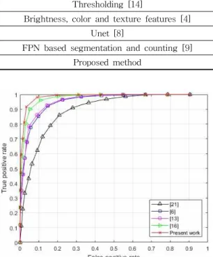
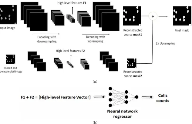
Cell segmentation and counting represent one of the most important tasks required in order to provide an exhaustive understanding of biological images. Conventional features suffer the lack of spatial consistency by causing the joining of the cells and, thus, complicating the cell counting task. We propose, in this work, a cascade of networks that take as inputs different versions of the original image. After constructing a Gaussian pyramid representation of the microscopy data, the inputs of different size and spatial resolution are given to a cascade of deep convolutional autoencoders whose task is to reconstruct the segmentation mask. The coarse masks obtained from the different networks are summed up in order to provide the final mask. The principal and main contribution of this work is to propose a novel method for the cell counting. Unlike the majority of the methods that use the obtained segmentation mask as the prior information for counting, we propose to utilize the hidden latent representations, often called the high-level features, as the inputs of a neural network based regressor. While the segmentation part of our method performs as good as the conventional deep learning methods, the proposed cell counting approach outperforms the state-of-the-art methods.

Key words: Bio-cell Informatics, Cell Segmentation, Cell Counting, Pyramidal Convolutional Autoencoder, Artificial Neural Network

※ Corresponding Author : Ki-Ryong Kwon, Address:

(608-737) 599-1, 45 Yongso-ro, Namgu, Busan, Korea, TEL : +82-51-629-6257, FAX : +82-51-629-6230, E-mail : [email protected]

Receipt date : Nov. 6, 2018, Revision date : Dec. 6, 2018 Approval date : Dec. 10, 2018

††

Dept. of IT Convergence and Application Engineering, Pukyong National University

(E-mail : [email protected])

††

Dept. of Information & Communication Eng., Tongmyong University (E-mail : [email protected])

††††

Dept. of Information Security, Tongmyong University (E-mail : [email protected])

††††

Dept. of IT Convergence and Application Engineering, Pukyong National University

※ This work was supported by Basic Science Research

Program through the National Research Foundation of

Korea (NRF) funded by the Ministry of Science and ICT

(No. 2016R1D1A3B03931003, No. 2017R1A2B2012456) and

MSIT (Ministry of Science and ICT), Korea, under the

Grand Information Technology Research Center support

program (IITP-2018-2016-0-00318) supervised by the

IITP (Institute for Information & communications Tech-

nology Promotion)”.

elements being lost. It ends up with many of the cells being joined (connected) and causing a lack of spatial consistency. This is a very critical sit- uation as the full understanding of the images de- mands clear and fair results in terms of cells preservation. This fact explains why most of these traditional computer vision based methods demand quite intensive post-processing tasks [3].

Instead of using computer vision based methods, the literature has widely adopted the machine learning methodology. Following the classic two steps of a machine learning framework (feature extraction and classification), the pixels are repre- sented by their corresponding features and are used as the inputs of the classifier [4]. The features can be the intensity variation, the texture related information, the spatial characteristics or a mixed of all of them [4]. Also, different kinds of learning algorithms can be adopted, from the use of support vector machine (SVM) [5] to the artificial neural network (ANN) based classifiers [6]. The draw- back with these methods is that they suffer from the lack of the spatial consistency between the pixels. And, moreover, as for the computer vision based methods, they still require a lot of post-processing tasks that can be very expensive in terms of time.

Deep learning [7] based methods have gained attention in the recent years for their ability of un- derstanding images in a high-level fashion. Instead of using conventional machine learning methods with engineered features, researchers have widely adopted the deep learning methodology, which pro- vides a fully automated feature learning process.

Instead of manually choosing the features, the deep networks provide high-level feature processes learned in an automatic way [7]. They were also adopted in cell segmentation problems [8,9].

While most of them perform fairly pleasant seg- mentation, deep learning methods face the problem of the trade-off between the semantic and spatial features [9]. While the network gets deeper, it ex-

tracts more complex features that can recognize complex shapes and forms, but the fact of down- sampling the image while its goes through the net- work causes the loss of spatial consistency be- tween the pixels located in some regions of the images.

This leads to excellent results in terms of object recognition but unfair results in terms of shape and boundary preservation. And when it comes to mi- croscopy data, the preservation of the shape and the boundaries of the cells are more than neces- sary, they are critical. To tackle this trade-off problem, many studies have adopted the use of convolutional autoencoders (CAE), which do not simply map some given inputs to the class scores, but, instead, they try to construct a predefined seg- mentation mask given a certain input.

Beside the segmentation task, cell counting con- sists of estimating, using the input microscopy im- age, the number of the cells located inside it. Cell counting can be linked with the segmentation scheme in a one-network-to-tasks fashion [10], where a single network is used in order to produce the segmentation mask and to estimate the number of the cells in the same time. Or, cell counting can be investigated separately with segmentation [10], where, again, the segmentation mask is utilized separately for estimating the number of the cells inside it.

We propose a cell segmentation and counting

scheme which uses deep convolutional autoen-

coders (CAE) in a pyramidal way in order to dras-

tically encode the spatial resolution of the cells with

a high-level feature learning. First, inputs of dif-

ferent sizes are given to different CAEs for a

scale-based encoding-decoding system. Gaussian

pyramid representation is applied over the original

cellular images in order to generate inputs with

different size and different spatial resolution. Two

sizes are adopted in this work, the first input being

the original microscopy image, and the second in-

put being the Gaussian blurred and down-sampled

version. Each one of them is given to a different CAE which learns to construct the segmentation mask. The obtained masks from the two CAEs are summed in an element-wise fashion in order to produce the final segmentation mask.

The second step, the counting cell process, rep- resents the main contribution of this paper. We propose a novel cell counting method based on the utilization of the high-level features from the two CAEs and a shallow regressor network. The qua- si-majority of the papers in the literature propose the use of the generated masks as prior information for the cell counting. But, these constructed masks are generally noisy and do not provide accurate in- formation, especially in case of overlapping cells.

We avoided using the segmentation mask, as all the other papers do, but, in a quite original way, we propose to extract the latent representations of the images from the two CAEs. The extracted rep-

resentations are concatenated in one single feature vector, which will be used as the input of a neural network based regressor that will learn to output the number of the cells in the image.

We assume that the scale-dependent high-level feature learning process done with the pyramidal CAEs will allow the latent representations to stat- ically encode the shape, boundary and number of the cells and provide a better learning capability to the regressor. The results demonstrate that the proposed pyramidal CAE performs at least as good as the other state-of-the-art segmentation meth- ods in terms of cellular shape preservation. But, the proposed cell counting scheme achieves outstand- ing results and outperforms the conventional and other state-of-the-art methods that utilize the segmentations masks as prior information. Fig. 1 represents schematically the proposed method of this paper.

(a)

(b)

Fig. 1. Summary of the proposed Pyramidal CAE: (a) the construction of the segmentation masks with different input

sizes; (b) the features F1 and F2 are concatenated to form the high-level feature vector that will be used

as the input of a neural network based regressor for the cell counting part.

2. PROBLEM PRESENTATION

As explained before, the cell segmentation prob- lem consists of assigning every single pixel inside the microscopy image to the cells body or the background. The ground truth, which is commonly represented as a binary image in case of a binary classification, represents the expected segmenta- tion result, constructed by a manual labelling from biological experts. While building the dataset for the supervised learning process, the ground truth image is used as a label source for the pixels. In Fig. 2, we show some of the images used for the present work. In the left part of Fig. 2, we see the image resulting directly from the microscopy. In real world application, these kinds of images are instantaneously used for the purpose of analysis, and, consequently, any segmentation scheme must be able to analyze it. We can guess how difficult it can be to segment such a very low contrast image. That image contains 14 cells, the one shown in the center also contains 14 cellular elements. The image shown in the right of Fig. 2 contains 100 cellular elements.

Patch-based segmentation is the process of rep- resenting each pixel by a small square of a given n×n size, called patch, with the concerned pixel, the one that must be classified, located right in the center of the square image, being surrounded by the neighboring pixels. The label that must be as- signed to the center pixel is seen as the label of all the patch. Which means that every data will be

a really small image with the concerned pixel in the middle. The CAE does not involve the patch creation, since the images are given in their origi- nal size. The next two sections present step by step the proposed method

3. SEGMENTATION WITH PYRAMIDAL CAE Auto-encoders [11] are unsupervised learning methods that are used for the purpose of feature extraction and dimensionality reduction of data.

Neural network based auto-encoder consists of an encoder and a decoder. The encoder takes an input x of dimension d, and maps it to a hidden repre- sentation, of dimension r, using a deterministic mapping function f such that

(1) where the parameters W and b are the weights and bias associated with the layer that takes the input x. These parameters must be learned by the en- coder system. The decoder then takes the output y of the encoder and uses the same mapping func- tion f in order to provide a reconstruction f that must be of the same shape or in the same form (which means, almost equal to) as x. Using equa- tion (1), the output of the decoder is also given by (2) where the parameters W’ and b’ are the weights and bias associated with the decoder layer. In final, the network must learn the parameters W, W’, b and b’ so that z must be close or, if possible, equal

Fig. 2. Examples of the images used for the experiments: left, a microcopy image containing 14 cells; in the center,

we have 14 cells also; in the right, the image contains 100 cells. We can remark how the complexity of the

task augments as the number of cells increases.

to x. Though, the network leans to minimize the differences between the input x and the decoder’s output z.

This encoding-decoding process can be done with the use of convolutional neural networks, us- ing what we call the convolutional autoencoder (CAE). Unlike conventional neural networks, where you can set the size of the output that you want to get, the convolutional neural networks are char- acterized by the process of down-sampling, which is accomplished by the pooling layers, a down- sampling system that is incorporated in their architecture. As explained in the first section of the paper, this down-sampling process insidiously in- duces the loss of spatial information while we go deeper inside the network, causing the trade-off between the semantic and the spatial features.

In order to tackle this problem, we can use the CAE instead of conventional convolutional neural networks. In fact, in the CAE, after the down-sam- pling process accomplished by the encoder, the de- coder tries to up-sample the representation until we reconstruct the original size. This can be made by the so-called backwards convolution, often called “deconvolution” operations. In the segmen- tation process, instead of reconstructing the origi- nal input, like normal autoencoders do, we aim to reconstruct the segmentation mask when the net- work takes the original image. So, the final solution of the network can be written in the form

(3) where z still denotes the decoder’s output and m is the segmentation mask. This equation means that the network must learn the adequate parame- ters so that the difference between the decoder’s output z and the segmentation mask m is mini- mized. The adopted cost function is a cross-en- tropy cost described as

(4) where N represents the total number of data (total number of images used during the training proc-

ess), m still represents our segmentation mask, which is given by the ground truth, and z is the output of the decoder described in equation (2). The network learns the parameters in equation (3) so that the error in equation (4) is minimized.

In order to statistically embed the spatial in- formation of the input and to prevent the afore- mentioned trade-off between the semantic and spatial features, we propose, as discussed before, a pyramid of convolutional autoencoders. The idea is to use two CAEs with each one of them having an input size of different scale. The original scale will be used to encode the semantic features, and the decreased scale will be useful for the encoding of the spatial features. Gaussian pyramid is used in order to generate inputs of different sizes with different spatial resolution, as we show in Fig. 3.

As clearly illustrated in Fig. 1, the original image will be given to one of the CAEs and the down- sampled and blurred version will also be given to another CAE for the pyramidal feature learning solution. The final mask will result on the summa- tion of the two “reconstructed” masks from both CAEs. The second mask, which is the mask out- putted by the CAE that takes the down-sampled and blurred version, will be up-sampled in order to equal the original size and will be summed up with the mask outputted by the first CAE. The mask resulting from the summation will represent the final segmentation mask of the scheme. The

(a) (b)

Fig. 3. (a) An original image with 10 cells (520×696);

(b) the Gaussian blurred and down-sampled version, also containing 10 cells (260×348).

The Gaussian filter used here has a standard

deviation of 6.

architecture of the first CAE is shown in Table 1.

This architecture is the same with the one of the down-sampled version, but with all the dimensions divided by two, as we can clearly see in Table 2.

The two CAEs constitute what we call the pyr- amidal convolutional autoencoder, as they take two inputs of different scales and their outputs are summed in order to obtain one final segmentation mask. It is necessary to mention that, as we can see in the architecture of the two networks, the original image size (520×696, as depicted in Fig.

3), was first resized to 224×224. Thus, the down- sampled version has a size of 112×112.

In the two tables, we can see a process of down-sampling (encoding) with the stacking of many convolutional and pooling layers. Just after we reach a 1×1×4096 feature volume, we start the up-sampling process (decoding) with the stacking of many deconvolutional and unpooling layers. The convolutional layers are denoted by “Conv” in the tables, the pooling layers are mentioned by “Pool”,

the deconvolutional layers are represented by

“Deconv” and the unpooling layers are depicted as

“Unpool”.

4. NOVEL CELL COUNTING METHOD Each one of the 5

convolutional layers of the two CAEs contain 4096 neurons (1×1×4096). The activations from these layers are extracted and concatenated in order to form one single vector, which gives us 8192 dimensional final feature vec- tors. These vectors represent the latent repre- sentations of the CAEs and they are given to the neural network based regressor for the cell count- ing part. Which means that the second part of our proposed scheme, the cell counting part, starts by extracting the high-level features of the two CAEs. Then, we put them together in order to form one feature vector that contain the semantic and spatial characteristics of the input.

Unlike with classification, the network must

Table 1. CAE architecture for the original images.

Layer Filter size # Feature maps Stride Padding Output

Input - - - - 224224

Conv 1 33 64 1 1 224224

Pool 1 22 64 2 0 112112

Conv 2 33 128 1 1 112112

Pool 2 22 128 2 0 5656

Conv 3 33 256 1 1 5656

Pool 3 22 256 2 0 2828

Conv 4 33 512 1 1 2828

Pool 4 22 512 2 2 1414

Conv 5 1414 4096 1 1 11

Deconv 5 1414 512 1 1 1414

Unpool 4 22 512 2 2 2828

Deconv 4 33 512 1 1 2828

Unpool 3 22 256 2 0 5656

Deconv 3 33 256 1 1 5656

Unpool 2 22 128 2 0 112112

Deconv 2 33 128 1 1 112112

Unpool 1 22 64 2 0 224224

Deconv 1 33 1 1 1 224224

output a number designating the number of the cells that we have in the image. Artificial neural network (ANN) is an interconnected group of arti- ficial neurons. These neurons use a mathematical or computational model for information processing.

ANN is an adaptive system that changes its struc- ture based on information that flows through the network [12]. The neural network acquires the ability to generalize based on the training data and, if the training data contains all the characteristics, all the meaningful information possible of the proc- essed sounds or vibrations, the network can predict outcomes for new, previously unseen data sound or vibrations. One of the commonly used structures of ANN is the multi-layer perceptron. Using su- pervised learning, the sample {x

} is fed to the net- work and produces an output {y}. The input pattern {x

} is then propagated through the network in the following way:

(5)

where y

denotes the output of a given neuron i, and N the number of input neurons, while M de- notes the number of hidden layers. is the weighted sum in this form: j represents the input neuron that comes to feed the neuron, and n de- notes the layer where we are (n=1 represents the first layer). To implement this procedure, one needs to calculate the error derivative with respect to weight in order to change the weight by an amount that is proportional to the rate at which the error changes as the weight is changed. The backpropagation algorithm [12] is used in this re- search paper. The activation function f is a sigmoid function and is defined as:

(6) Once we have our feature vectors, we can con- struct our ANN based regressor. The network has an input layer containing 8196 neurons. We have created two hidden layers. The first one contains 250 neurons and the second one has 50 neurons.

The last layer contains one single neuron that must output the number of the cells located inside the Table 2. CAE architecture for the down-sampled and blurred version of the inputs.

Layer Filter size # Feature maps Stride Padding Output

Input - - - - 112112

Conv 1 33 64 1 1 112112

Pool 1 22 64 2 0 5656

Conv 2 33 128 1 1 5656

Pool 2 22 128 2 0 2828

Conv 3 33 256 1 1 2828

Pool 3 22 256 2 0 1414

Conv 4 33 512 1 1 1414

Pool 4 22 512 2 2 77

Conv 5 77 4096 1 1 11

Deconv 5 77 512 1 1 77

Unpool 4 22 512 2 2 1414

Deconv 4 33 512 1 1 1414

Unpool 3 22 256 2 0 2828

Deconv 3 33 256 1 1 2828

Unpool 2 22 128 2 0 5656

Deconv 2 33 128 1 1 5656

Unpool 1 22 64 2 0 112112

Deconv 1 33 1 1 1 112112

image. Which gives us a structure of 8196-250- 50-1. All the hidden layers use the squashing sig- moid function denoted in equation (6). But, because we face a regression problem here, and not a clas- sification one, the last layer has the rectified linear unit (ReLu) as the activation function. The ReLu is defined by:

(7) where z represents the outputs from the second hidden layer. The next section discusses about the obtained results using the proposed method.

5. RESULTS AND DISCUSSION

5.1 Segmentation

We have used the BBBC005 dataset from the Broad Institute’s Bioimage Benchmark Collection [20]. This dataset is a collection of 9,600 simulated microscopy images of stained cells. We have shown an example of these images in Fig. 2. The Institute has used the SMCEP simulation platform in order to generate these images. The cell were generated in such a way that they are similar to the U2OS human cells. The simulated cells were then blurred with variable Gaussian filters in order to mimic the phase microscopy temper. Each image in the data- base has a size of 520×696, and they are encoded in 8-bit grayscale. As explained before, for the purpose of using these images in our networks, we have resized them to 224×224. Among the 9,600 images, 1,200 have their ground truth labelled by hands. These ground truths, as explained before, are utilized as the label source for the feature learning process. Among the 1,200 images that have ground truths, 700 were utilized as the train- ing data. The results concerning the projections of the features extracted from the CAEs are shown in Fig. 4 and we can see how discriminative they are. By discriminative, we mean that they can be easily separated by a strong nonlinear classifier, explaining why most of the segmentation masks are really pleasant.

It is necessary to mention that the segmentation result radically depends on the nature of the image under investigation. In case of non-overlapping cells, and when the image contains between one and around 30 cells, the results obtained using our proposed method and the deep learning based state-of-the-art methods are quite similar. It is very difficult to see any differences between them.

In fact, in Fig. 5, we show the results concerning the segmentation for the case where the image does not contain overlapping cells. And the image in Fig. 5 contains only 18 cellular elements. In Fig.

5 (a), we have the original phase contrast image, in (b), we have the ground truth, in (c) we have the result obtained by using our method, in (d) we have the result using the Unet [8] and, finally, in (e), we show the result using the FPN as proposed in [9]. We can remark that all the results are equiv- alent and they are very outstanding because they produce almost the same result than the ground truth.

But, in case of overlapping cells and when the image contains many elements, the differences be- tween the three methods becomes slightly clear. In Fig. 6, we show the results in case of overlapping cells and the image contains 35 cells. The regions marked in red in the results denote the cases where Fig. 4. Visualization of the latent representations ex-

tracted from the networks.

the cells are connected. The image shown in Fig.

6 (c), which is the result of our method, has less marked regions compared to the others, which

means less connected cells.

For an objective evaluation and comparison of the segmentation result, we have computed the

(a) (b) (c)

(d) (e)

Fig. 5. Results of the segmentation, case of non-overlapping cells. (a) The original phase contrast image; (b) the ground truth; in (c), (d), and (e), we have the masks computed using the proposed method, the Unet [8] and the FPN [4], respectively. The image contains 18 cells.

(a) (b) (c)

(d) (e)

Fig. 6. Results of the segmentation, case of overlapping cells. (a) The original phase contrast image; (b) the ground

truth; in (c), (d), and (e), we have the masks computed using the proposed method, the Unet [8] and the FPN

[4], respectively. The image contains 35 cells.

dice similarity index (DSC) of the final segmenta- tion mask. This index computes the difference be- tween the ground truth and the segmentation result in terms of region ratio. The DSC is denoted in equation (8), where A

denotes the targeted re- gions (in our case, the cell interior) of the ground truth, while A

denotes the segmented region us- ing the proposed scheme. The operator | ■ | com- putes the number of pixels in the given region.

(8)

The DSC is a number between 0 and 1, DSC

∈ [0 1], and when it is close to 1 it means that the segmented result is very similar to the targeted or expected result (ground truth), and when it is close to 0, it means that the segmented result and the ground truth are really different. A greater DSC denotes a good segmentation and a small one de- notes a poor segmentation. Another index is the Jaccard index (JI), computed by

(9) which is the intersection between ground truth and the segmented region divided by the union of the two regions.

We conduct a comparison study with the method in [16], where the authors have used a feature pyr- amid networks but with two big differences: first, they have down-sampled the original input without using Gaussian pyramid, like proposed here; sec- ondly, as most of the conventional methods in the cell counting literature, they have used the mask generated by the network as the prior information for counting the cells. We demonstrate here that using the latent representation of the networks in- stead of utilizing the created masks, which contain significant noisy information, can lead to better results. Another method using the deep learning based approach can be seen in [8]. The difference is not important since all these methods, in terms of segmentation, accomplish better results com-

pared with traditional computer vision and machine learning methods. Our proposed segmentation meth- od also accomplishes as good results as the two deep learning methods.

We have, using our method, a DSC of 0.96, whereas the method in [9] stagnates at 0.95. Same with the JI index, where our method is slightly better. The reason comes from the fact of utilizing different spatial resolution provided by the Gaus- sian pyramid in our case. The Unet in [12] accom- plishes 0.93 and 0.86 for the DSC and JI, re- spectively.

The computer vision based method, the dynamic thresholding proposed by Otsu [13 ] cannot seize the cellular properties and leads to the significant lack of consistency. Using the thresholding method requires an intensive post-processing task. The post-processing can be the use of multiple mor- phological operations and different thresholding methods again, costing a lot of time to the user.

The DSC and JI stagnate at 0.75 and 0.62, re- spectively, for this computer vision based conven- tional method.

The conventional machine learning method used for the comparison is the method developed in [4].

In this work, the authors have proposed the su- pervised-learning based segmentation using the brightness, color and texture features. This method also lacks the spatial consistency and requires, as for the dynamic thresholding method [14], a lot of post-processing burden. All the results are sum- marized in Table 3.

Another objective comparison for the segmenta-

tion results is shown with the ROC-curves of the

classification, computed in a pixel level and shown

in Fig. 7. As mentioned before, the difference is

not too much between the deep learning methods,

even though our proposed scheme performs slight-

ly better. The computer vision and the conventional

machine learning based methods perform a bit

poorly, since they require a lot of post-processing

task, as explained in the previous paragraph.

Fig. 7. ROC-curves for the classification of the pixels of the different methods.

5.2 Cell counting

As said before, we propose a very novel method for counting the cells by using, not the segmented masks, as most of the methods do, but the latent representations learned by the deep pyramidal CAEs. As we have seen with the segmentation re- sults presented in the previous section, the seg- mentation masks are always noisy because they increase the connections between the cells when the image contains many overlapping elements. This is the principal reason why we have avoided to use the outputted masks as the prior information for counting the cells. Instead, we propose in this paper to utilize the high-level features learned by the two CAEs as the inputs of a neural network based regressor.

In Fig. 8, we show the results concerning the counting part. We show the actual number of the cells, provided as a ground truth, and the number

computed by three different methods. The results for the computer vision based techniques for the cell counting, as proposed in [15], are shown in green. The results for the state-of-the-art deep learning method, as used in [9], are shown in magenta. And our results are shown in red color.

As we can see in Fig. 8, the more we have cells in the image, the more difficult is to predict the exact number of the cells, because when there are too many cells in the image, the probability of also having many overlapping cases is really high. But, if we look at Fig. 8, we see that our method man- ages to stay close to the “actual number of cells”, shown in blue color. Even when the number of the cells goes really high, our proposed method still manages to output values that are really close to the real number of cells. And, in case we have less than 30 cells, as we can see in the Fig. 8, our meth- od performs without an error. In the same time, Table 3. DSC and JI indices values.

Method DSC JI Post-processing

Thresholding [14] 0.75 0.62 Intensive

Brightness, color and texture features [4] 0.88 0.74 Intensive

Unet [8] 0.93 0.86 Not intensive

FPN based segmentation and counting [9] 0.95 0.86 Not intensive

Proposed method 0.96 0.87 Not intensive

Fig. 8. Relation between real and predicted number of

cells for the 3 methods.

we see how the computer vision based techniques really fail when the number of the cells surpasses 30. The state-of-the-art method also has some difficulties when the number of the cells increases.

In Fig. 9, we show the differences between the real number and the computed number of the cells.

The difference is computed by comparing the ac- tual number of the cells in the image and the counted number, as described by the following equation

(10) where RN is the real number of the cells provided by the ground truth and ON represents the number outputted by the classifiers. As we can strongly remark in Fig. 9, the divergence between our pre- dicted numbers and the real values starts at 40 cells. But, still the difference is around 2, which is really small. We clearly see that the complexity of the counting problem increases at the same time as the number of the cells.

But, in the opposite way, the fact of using the segmentation masks as prior information for counting the cells really depreciates the accuracy of the regressor, as we can remark with the results of the state-of-the-art deep learning based method proposed in [9]. When we surpass the 30 cells, the divergence between the actual number of cells and

the predicted number of that method is really important. This is a critical point where our method shows better improvement. As we could have ex- pected, the divergence is really high for the com- puter vision techniques used in [15].

Another comparative study can be seen in Fig.

10 where we show the prediction error of the three different methods. This evaluation metric was computed by using the following equation

(11) where RN is the real number of the cells provided by the ground truth, ON represents the number outputted by the classifiers. We can see that our proposed method (2.18 % of prediction error) out- performed the conventional computer vision based method (22.32 %) and also the state-of-the-art deep learning method (7.99 %).

6. CONCLUSION

Segmentation is one of the most important steps for the fully understanding of images of biological processes. We have proposed a segmentation scheme of the biological images. We have used a pyramidal deep convolutional autoencoder in order to reconstruct the segmentation masks. And we have proposed a novel cell counting method by us- Fig. 9. Difference between real and predicted number

of cells for the 3 methods. Fig. 10. Prediction error of the three methods.

ing the latent representations learned by the net- work as the inputs of a neural network based regressor. Our method significantly reduces the trade-off between the semantic and spatial fea- tures by allowing to capture features from different scales. The results show that the proposed method can perform a very pleasant segmentation and, most importantly, outperforms the state-of-the- art method in case of cell counting.

REFERENCES

[ 1 ] O. Sliusarenko, J. Heinritz, T. Emonet, and C.

Jacobs-Wagner, “High-Throughput, Subpixel Precision Analysis of Bacterial Morphogen- esis and Intracellular Spatio-Temporal Dyna- mics,” Molecular Microbiology, Vol. 80, No.

3, pp. 621-627, 2011.

[ 2 ] J.W. Young, J.C.W. Locke, A. Altinok, N.

Rosenfeld, T. Bacarian, P.S. Swain, et al.,

“Measuring Single-Cell Gene Expression Dynamics in Bacteria Using Fluorescence Time-Lapse Microscopy,” Nature P rotocols, Vol. 7, No. 1, pp. 80-88, 2012.

[3 ] S. Tay, J.J. Hughey, T.K. Lee, T. Lipniacki, S.R. Quake, M.W. Covert, et al., “Single-Cell NF-κB Dynamics Reveal Digital Activation and Analogue Information Processing,” Nature, Vol. 466, No. 7303, pp. 267-271, 2010.

[ 4 ] D.R. Martin, C.C. Fowlkes, and J. Malik,

“Learning to Detect Natural Image Bounda- ries Using Local Brightness, Color, and Tex- ture Cues,” IEEE Transactions on Pattern Analysis and Machine Intelligence, Vol. 26, No. 5, pp. 530-549, 2004.

[ 5 ] N. Madusanka, Y.Y. Choi, K.Y. Choi, K.H.

Lee, and H.-K. Choi, “Hippocampus Segmen- tation and Classification in Alzheimer’s Dis- ease and Mild Cognitive Impairment Applied on MR Images,” Journal of Korea Multimedia Society, Vol. 20, No. 2, pp. 205-215, 2017.

[ 6 ] A.E. Carpenter, T.R. Jones, M.R. Lamprecht,

C. Clarke, I.H. Kang, and O. Friman, et al.,

“CellProfiler: Image Analysis Software for Identifying and Quantifying Cell Phenotypes,”

Genome Biology, Vol. 7, No. 10, pp. r100-r100, 2006.

[ 7 ] Y. LeCun, Y. Bengio, and G. Hinton, “Deep Learning,” Nature, Vol. 521, pp. 436-444, 2015.

[ 8 ] O. Ronneberger, P. Fischer, and T. Brox, “U- Net: Convolutional Networks for Biomedical Image Segmentation,” Proceeding of Medical Image Computing and Computer Assisted Intervention 2015, pp. 234-241, 2015.

[ 9 ] C.X. Hernandez and M.M. Sultan, “Using Deep Learning for Segmentation and Count- ing Within Microscopy Data,” arXiv e-prints arXiv:1802.10548, 2018.

[10] G. Ghiasi and C.C. Fowlkes, “Laplacian Pyramid Reconstruction and Refinement for Semantic Segmentation,” Proceeding of European Conference on Computer Vision, pp. 519-534, 2016.

[11] G.E. Hinton and R.R. Salakhutdinov, “Reduc- ing the Dimensionality of the Data with Neural Networks,” Science, Vol. 313, No. 5786, pp. 504-507, 2006.

[12] D.E. Rumelhart, G.E. Hinton, and R.J. Wil- liams, “Learning Representations by Back-Pro- pagating Errors,” Nature, Vol. 323, pp. 533- 536, 1986.

[13] V. Ljosa, K.L. Sokolnicki, and A.E. Carpenter,

“Annotated High-Throughput Microscopy Image Sets for Validation,” Nature Methods, Vol. 9, No. 7, pp. 637-637, 2012.

[14] N. Otsu, “A Threshold Selection Method from Gray-Level Histograms,” IEEE Transactions on Systems, Man, and Cybernetics, Vol. 9, No.

1, pp. 62-66, 1979.

[15] L. Putzu, G. Caocci, and C.D. Ruberto, “Leu-

cocytes Classification for Leukemia Detection

Using Image Processing Techniques,” Artifi-

cial Intelligence in Medicine, Vol. 62, No. 3,

pp. 179-191, 2014.

Caleb Vununu

He received his B.S. degree in Computer Science in Youngsan University, Republic of Korea in 2015. Since September 2015, he’s a Master degree student in the department of IT Convergence and Application Engineering in Pukyong National University. His research interests include Signal Processing and Machine Learning.

Kyung-Won Kang

He received a B.S., a M. S., and a Ph. D. degrees in Electronics Engineering in Pukyong Natio- nal University in 1996, 1998 and 2002 respectively. He worked at Homecat, a set-top box manu- facture from 2006-2014. He is currently an assistant professor in Department of in- formation and Communications Engineering at Tongmyong University. His research interests are in the are of digital image processing and machine learning.

Suk-Hwan Lee

He received a B.S., a M.S., and a Ph. D. degrees in Electrical Engineering from Kyungpook National University, Korea in 1999, 2001, and 2004 respectively.

He is currently an associate professor in Department of Infor- mation Security at Tongmyong University. His re- search interests include multimedia security, digital image processing, and computer graphics.

Ki-Ryong Kwon

He received the B.S., M.S., and Ph.D. degrees in electronics en- gineering from Kyungpook Natio- nal University in 1986, 1990, and 1994 respectively. He worked at Hyundai Motor Company from 1986-1988 and at Pusan Univer- sity of Foreign Language from 1996-2006. He is cur- rently a professor in Department of IT Convergence and Application Engineering at the Pukyong National University. He has researched University of Minnesota in USA in 2000-2002 with Post-Doc. and Colorado State University on 2011-2012 with visiting professor.

He was the President of Korea Multimedia Society in

2015-2016. His research interests are in the area of

digital image processing, multimedia security and wa-

termarking, bioinformatics, weather radar information

processing, and machine learning.