Mapping the Geographic Variations of the Low Birth Weight cases in South Korea: Bayesian Approaches
Young-hee Roh* · Key-ho Park**
우리나라 저체중아 출생의 공간적 변동성 지도화: 베이지언적 접근
노영희*·박기호**
Abstract : This study reviewed and compared methods for mapping aggregated low birth weight (LBW) and geographic variations in LBW in South Korea. Based on this review, we produced LBW maps in South Korea.
Standardized mortality/morbidity ratios (SMRs) and crude mortality rates have been widely used for many years in epidemiological research. However, SMR-based maps are likely to be affected by sample size of unit area. Therefore, this study adopted a model-based approach using Bayesian estimates to reduce noisy vari- ability in the SMR. By using a Bayesian model, we can calculate a statistically reliable RR values. We used the full Bayes estimator, as well as empirical Bayes estimators. As a result, variations in the two Bayes models were similar. The SMR-based statistics had the largest variation. The result maps can be used to identify regions with a high risk of LBW in South Korea.
Key Words : spatial epidemiology, spatial statistics, bayesian analysis, disease mapping, low birth weight (LBW), standardized mortality/morbidity ratio (SMR)
요약 :본 연구에서는 우리나라에서 발생한 저체중아 출생 집계 자료를 공간적으로 지도화하기 위한 기법들
을 검토·비교하고, 이를 기반으로 우리나라의 LBW 지도를 작성하였다. 표준화사망률이나 조사망률 등은 역 학 분야에서 지속적으로 광범위하게 사용되고 있는 지표이다. 그러나 이러한 표준화사망률은 집계 단위의 샘 플 수에 영향을 많이 받는다는 단점을 가지고 있다. 이에, 본 연구에서는 베이지언 기법을 활용하여 샘플 수에 따른 통계적 변동성을 감소시키고자 하였다. 이를 위해 경험적 베이지언 기법과 풀 베이지언 기법을 모두 활용 하였고, 결과적으로 유사한 통계량을 산출한 것을 확인할 수 있었다. 반면, SMR 기반의 통계량은 높은 분산을 가지고 있음을 확인하였다. 연구의 결과에 따른 통계 지도는 우리나라 저체중아 출생의 높은 위험도를 가지는 지역들을 파악할 수 있도록 한다.
주요어 :공간역학, 공간통계, 베이지언 분석, 질병 지도화, 저체중아, 표준화(유병률)사망률
* Invited Research Fellow, Division of Natural Resources Conservation, Korea Environment Institute, [email protected]
** Professor, Department of Geography, Seoul National University, [email protected]
1. Introduction
According to data from the Ministry of Health and Welfare in South Korea (2012), the proportion of low birth weight (LBW) and multiple births are increasing over time. Between 2004 and 2010, LBW rates increased 25% from 4.1% to 5%. Ylppö (1919) originally defined LBW as infants weighing less than 2,500 grams. In 1950, the World Health Organization (WHO) adopted a fig- ure of less than 2,500 grams as a universal definition of LBW (WHO, 1950). LBW is a well-known risk factor for increased infant morbidity and mortality. LBW has become the second leading cause of death among infants, after premature birth (Valero De Bernabé et al., 2004).
By school age, children with a LBW are more likely than those with a normal birth weight to have mild learning disabilities, attention disorders, developmental impair- ments, and breathing problems, such as asthma (Shiono and Behrman, 1995).
Many studies have analyzed the potential risk factors for LBW including socio-economics, smoking, maternal age, and educational level (Chomitz et al., 1995; Rush and Cassano, 1983; Shiono and Behrman, 1995; Valero De Bernabé, 2004). Maternal age is considered as an im- portant determinant of birth outcome and is thought to represent a mother’s biological or psychosocial prepared- ness for childbearing (Geronimus, 1996). Mothers over 35 years old have a higher chance to get a LBW infant when it compares to mothers aged 20 to 29 years old (Berkowitz et al., 1990). According to the Bureau of Sta- tistics in South Korea (2015), the average age for a person to marry has been increased in recent years. The age for a man’s marriage was 32.4 years in 2014, up from 29.3 in 2000. In addition, the age for a woman’s marriage was 29.8 years in 2010, up from 26.5 in 2000. Reasons for delayed marriage include trends for increasing number of women with active participation in economic and social fields, high educational level of women, and changing
social attitudes to marriage. Under the current circum- stances, the average maternal age has also been increased.
According to Song and Choi (1999), the average ma- ternal ages in South Korea were 27.9 and 30.8 in 1995, 2008, respectively. They also reported that the propor- tion of advanced maternal age women in South Korea in- creased about three times between 1995 and 2008 (4.7%
to 14.3%).
The research on LBW in South Korea has been pre- dominantly focused on causes of LBW and developmen- tal problems associated with LBW rather than disease mapping. Maps can depict the incidence and relative risk (RR) rates of LBW with visualization techniques.
Disease mapping can also be utilized to assess our needs for health alerts or to formulate hypotheses and models involving potential covariates. Using a series of statisti- cal choropleth maps, we examined the geographical patterns of LBW in South Korea. When calculating the RR for the area-specific aggregated data, we have to pay attention to the variance of RR according to the sample size. SMR is calculated by the ratio of the observed value divided by the expected value. Therefore, if the number of sample is small, SMR statistics have large variance. To compensate for this point, we calculate statistically reli- able RRs by utilizing the Bayesian techniques. The study that utilizes Bayesian techniques in epidemiological field can be found in the Roh and Park (2014).
In Section 2, we present a spatio-temporal overview and descriptive statistics of birth counts. Then, we provide a brief review of the statistical methods used to estimate epidemiological rate values, such as RR rates.
Bayesian model-based estimates are discussed in detail.
In the next section, we calculated statistically reliable risks using Bayesian model-based estimates such as Pois- son-Gamma and full Bayes model. The results of calcula- tion were used to produce statistically reliable risk maps.
In addition, we made the difference maps between SMR and Bayesian model-based methods.
2. Materials and Methods
1) Materials
Vital statistics on births were obtained from the birth records of the National Statistical Office, South Korea.
Each record contains information on infants, such as date of birth, location, weight, sex, and data on mothers including education, job, and age. The temporal range of this study encompassed 3 years from the beginning of January 2008 to the end of December 2010. LBW data- sets were spatially aggregated according to geographical units. South Korea consisted of 249 Si-Gun-Gu levels of administrative districts in 2009. Th e average area of these districts is about 402 km2, but each area of district has a great diff erence. For example, Jung-Gu within the Busan is the smallest of the districts (3 km2), and Hongcheon- gun within the Gangwon-do is the largest (1,817 km2).
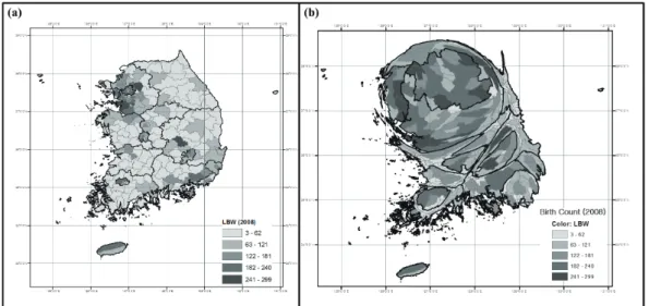
Utilizing a variety of area information, we can create a cartogram. Cartogram is one of the effective mapping techniques to present statistics with distortion of area information of each region. By taking advantage of the
cartogram, we can easily compare the statistics of each region with amount of distortion. By doing so, we can detect the regions where have high risk values. As shown in cartogram in Figure 1, birth counts show a great range of variability throughout the areas. We made maps of LBWs in 2008 (panel (a)) and cartogram of newborn ba- bies with the same coloring scheme in (a) (panel (b)). Th e legends in (a) and (b) are the same. As shown in the carto- gram (b), birth counts in South Korea were concentrated in metropolitan areas and major cities include Gwangju, Busan, and Daegu. The birth counts, LBW cases, crude rates, and SMR of each administrative area are summa- rized in Table 1. LBWs seemed to increase slightly during the three years. Th e crude birth rate indicates the number of live births per 1,000 populations per year. Based on crude rates, 50 newborn babies were classifi ed as LBW on average (approximately 5%). SMRs are commonly com- puted in the field of spatial epidemiology. The SMR is a ratio of the observed count within an area to the expected count based on the “at-risk” population (Lawson, 2006).
A ratio greater than 1.0 suggests an excess risk. SMR had a range of values from 0.11 to 2.13 in 2009.
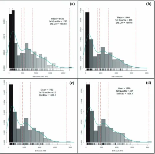
Figure 2 represents histograms and density plots of the
Figure 1. Maps of LBW in South Korea ((a) The number of LBW in South Korea, (b) Cartogram of birth counts)
birth counts in 2008, 2009, 2010, and 3 years data. In each plot, x axis represents the number of newborn baby and y axis represents the density of newborn baby. As
seen in the graph, the distribution of the number of new- born baby does not follow a normal distribution. There are many areas with small number of newborn baby.
Figure 2. Birth counts in South Korea ((a) counts of 3 year aggregates, (b) 2008, (c) 2009, (d) 2010.
The darkest bar represents 1st quartile range and the dotted line represents quintiles, the dashed line represents mean, and the curve represents the density)
Table 1. Descriptive statistics of birth count
Statistics Birth counts LBW cases Crude rate* SMR
2008 2009 2010 2008 2009 2010 2008 2009 2010 2008 2009 2010
minimum 76 63 50 3 1 2 16 5 24 0.331 0.110 0.476
median 1592 1453 1632 73 74 79 48 49 50 1.003 0.997 0.992
mean 1871 1787 1888 91 88 95 50 50 50 1.028 1.020 1.000
maximum 6610 7542 8207 301 358 428 87 5 91 1.783 2.128 1.816
* Crude rate is per 1,000 babies
For these reasons, we have to use the statistically reliable model, such as Bayesian model-based estimates to calcu- late the reliable relative risk.
2) Adjusting and transforming prevalence data
Observing the number of cases alone does not provide any information on the disease risk of a population. Ob- served values must be compared to expected values. The SMR is a common way to measure relative risks (RR).
A RR over 1 suggests an increased risk of that outcome in the exposed group. The SMR can be a useful approxi- mation of RR when the excess in mortality is consistent across all age groups (Symons and Taulbee, 1980). The SMR and its statistical significance are usually estimated and mapped for each region (Costello et al., 1974; Elsen et al., 1992; Meliker et al., 2007). However, estimates of SMRs often show a large variability. Small population areas tend to present extreme RR estimates, and it will stand out on the map (Bernardinelli and Montomoli, 1992). Incidence rates often suffer from the ‘Small Num- ber Problem.’ The variance of rate depends on the size of the denominator when the nominator is rare events. In the Small Number Problems, if the denominator is small, variance of rate will be large. If the denominator is large, variance of rate will be small. The Small Number Prob- lem occur various geographic areas where the population is sparse or the numerator is a rare event. If this occurs, small random fluctuations of variable may cause large fluctuations in the resulting percentage, ratio, or rate (Kennedy, 1989).
To develop statistically robust model-based estima- tions, researchers have been utilized information from global mean and Bayes approaches. Clayton and Kaldor (1987) proposed a model-based Bayesian approach.
According to this study, unknown RRs are modeled collectively as a spatial stochastic process. Since then, a number of related studies have been published (Marshall, 1991; Mollie and Richardson, 1991; Richardson et al.,
2004). According to Bayesian model-based approaches, each area has an estimated RR, which is a compromise between its SMR and inferences from information ob- tained from all of the areas combined. Such approaches reduce risk estimates and result in stabilized maps with better epidemiological interpretation (Bernardinelli and Montomoli, 1992). One way to account for spatial asso- ciations is to define a neighborhood in i-th area and to use the neighborhood to set prior parameters for θi; θi is the RR risk in i-th region. Then, θi is estimated by shrinking the disease rates toward the neighborhood mean, instead of a global mean (Marshall, 1991). The results of local shrinkage are produced by local estimators in each area.
(1) SMR
Due to the fact that it has simple computational pro- cedure, the SMR is the most widely used standardization statistic in risk ratio assessments in the field of public health. The SMR can be interpreted as a ratio of the ob- served to expected numbers of cases. The expected num- ber of case is determined by the standard population.
The average risk rate of a national aggregate population is often employed as a standard. The SMR is a maximum likelihood estimate of the RR under a Poisson model of the observed number of disease occurrences. Within a map of n regions, Oi denotes the observed case in i-th region, Ei is the expected count in i-th region, and θi is the RR risk in i-th region. We assume that the expected counts are known constants.
O‹ i = θi~Poisson(Eiθi) θi≡ SMRi =Oi/Ei
The observed count in the i-th region is assumed to be a Poisson distribution, with mean Eiθi, and the likeli- hood L(θ) and log-likelihood l(θ) of {Oi} is given by:
L(θ) =
Oi! exp(-Eiθi)
Пn {Eiθi}Oi =Пni Poisson(Oi; Eiθi)
L(θ) ∝П θn iOi·exp⎛-∑nEiθi
⎝ ⎞
⎠ l(θ) = lnL(θ) -∑Oilnθiv-∑Eiθi
(2) Bayesian methods
Empirical Bayes statistics are calculated using penal- ized log-likelihood maximization. Empirical Bayes information is derived from a model of a reference popu- lation. The full Bayesian method utilizes simulations of the joint posterior distribution. One of the strengths of this approach is that it allows for precise assessments of uncertainty. Instead of a point estimate of the expected mean and its variance, it generates a distribution of likely values using a prior distribution. This enables variance to be calculated more accurately (Persaud et al., 2010).
For example, in the following basic framework for a Bayesian analysis (Marshall, 1991), suppose that θ=(θ1,...,θn) are the risks to be estimated at N areas and y=(y1,...,yn) are the numbers of diseases in populations of size n1,...,nN. In the Bayesian approach, inferences about θ are based on the posterior distribution P(θ|y) of θ, which is obtained by combining the likelihood with the prior via Bayes’ rule (Carriquiry and Pawlovich, 2004).
As the posterior distribution is a product of a likelihood and prior distribution, it describes the behavior of param- eters after data have been observed and prior assumptions have been made. The posterior distribution is defined as follows:
P(θ|y) = C L(y|θ)g(θ) where C =⌠⌡pL(y|θ)g(θ)dθ
Where g(θ) is the joint distribution of the vector θ.
This distribution g(θ) can be specified as a proportional- ity, p(θ|y)∝L(y|θ)g(θ).
Computational problems have hindered the applica- tion of the full Bayes approach, but recent developments
in Bayesian analysis, mainly in the area of a Monte Carlo technique called the Gibbs sampler, provide a means of overcoming these difficulties. Clayton (1989) and Besag et al. (1991) proposed the application of the Gibbs sam- pler in disease mapping for the first time. Using the pos- terior distribution, we can compute points and intervals of estimates, thereby accessing uncertainty in risk maps.
Based on a comparison of empirical and full Bayes esti- mators, Bernardinelli and Montomoli (1992) concluded that the latter has advantages due to its ability to quantify uncertainty in parameters in the model.
To determine whether different estimators produce different values, we applied empirical and full Bayesian model-based approaches to RRs to calculate reliable risk statistics. To verify the level of stabilization, we depicted risk statistics, and compared variability of SMR and Bayes estimates through the difference maps.
3. Results
1) Geographical visualization of relative risks using an empirical Bayesian model
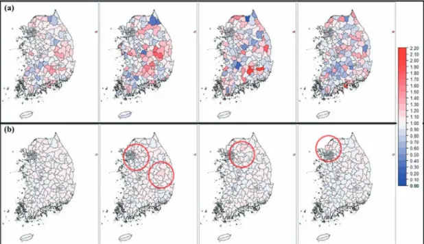
We calculated model-based SMRs using the Poisson- Gamma prior model of parameters. Figure 3 and 4 depict the maps produced with the empirical Bayes Poisson- Gamma model. For comparison, the SMR maps are in- cluded in this figure. In addition, the red circles indicate the high RR regions. We assume that the RRs {θi} are iid (independent and identically distributed) and they follow a gamma distribution with a scale parameter α and shape parameter ν. Conditional on θi, the observed deaths Oi are Poisson variates with expectation θiEi (Clayton and Kaldor, 1987). In Bayesian estimation, if there is small variance in the crude rate, then it will remain unchanged relatively. In contrast, if there is a large variance in the estimation of the crude rate, it will show strong shrink-
age toward the overall mean. For this reason, the map with the Poisson-Gamma estimator is shrunk toward the overall mean when it compares to a map of SMR.
As shown in Figure 3 and 4, empirical Bayes estimates
of RRs show smaller variations than the SMR. Extreme SMR estimates based on small populations have shrunk toward their global mean. However, extreme estimates based on large populations are maintained.
Figure 4. Maps of LBW relative risks - Enlarged map of the metropolitan area ((a) SMR - from the leftmost panel, 3 years aggregates, 2008, 2009, and 2010, (b) Poisson-Gamma estimates - 3 years aggregates, 2008, 2009, and
2010)
Figure 3. Maps of LBW relative risks ((a) SMR - from the leftmost panel, 3 years aggregates, 2008, 2009, and 2010, (b) Poisson-Gamma estimates - 3 years aggregates, 2008, 2009, and 2010)
In 2008, the SMR values were high in Uiseong-gun, Seongju-gun, Yecheon-gun, Geochang-gun, and Cheon- gyang-gun. In the empirical Bayes map, they were high in Dongdaemun-gu, Gwangju-si, Jung-gu (Ulsan), An- dong, Yangju-si regions. In 2009, SMR values were high in Cheongdo-gun, Hapcheon-gun, Yeongyang-gun, Ulleung-gun, Boeun-gun. Chuncheon-si, Seongnam- si Sujeong-gu, Seongnam-si Jungwon-gu, Daedeok-gu, and Icheon-si in the empirical Bayes map. In 2010, they were high in Namhae-gun, Jung-gu (Busan), Ulleung- gun, Hwacheon-gun, Goseong-gun regions. However, Bupyeong-gu, Paju-si, Nam-gu (Incheon), Jung-gu (Ulsan), Ulju-gun regions had high SMR values in the stabilized map. In the map with 3-year aggregated data, Ulleung-gun, Hapcheon-gun, Jung-gu (Busan), Uis- eong-gun, Geochang-gun regions had high SMR values.
However, in the empirical Bayes map, Jung-gu (Ulsan), Seo-gu (Daegu), Dongducheon-si, Nam-gu (Incheon), Gwangju-si regions had high SMR values.
2) Geographical visualization of the relative risks using full Bayesian modeling
Th e full Bayesian method uses a stochastic simulation technique called the Gibbs sampler, and the value of pos- terior distributions is obtained from the Markov chain Monte Carlo technique. We performed Gibbs sampling with a burn-in of 10,000 iterations, followed by 10,000 further cycles. We used 10,000 simulations of Markov chains after the 10,000 burn-in period to calculate the mean and median of the parameters. Figure 5 compares the various estimates obtained with the diff erent estima- tors in 2008. Th e Poisson-Gamma model and full Bayes- ian technique produced very similar estimates in all the regions. Some extreme RRs, which suff er from small at- risk population, were effectively attenuated to the prior global mean.
3) Comparison of the results
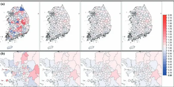
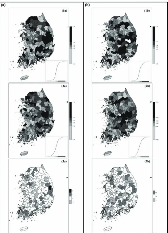
Table 2 and Figure 6 depict t h e quintile diff erences be- tween the SMR and the statistics of the Poisson-Gamma
Figure 5. Comparison of SMR, Poisson-Gamma, full Bayes mean and median in 2008 ((a) from the leftmost panel, SMR, Poisson-Gamma, full Bayes mean and full Bayes median, (b) Enlarged map of the metropolitan area)
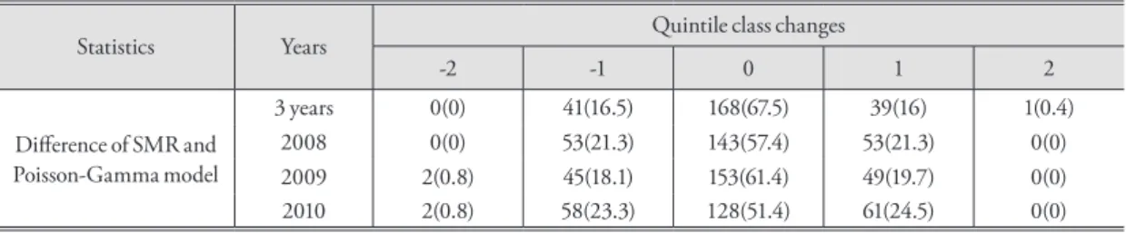
model. After calculating the SMRs and the statistics of Poisson-Gamma model, the regions were assigned to specific quintile classes according to their RRs. We calculated the differences in the quintile classes between SMR and the statistics of Poisson-Gamma model. As in the research of Pickle and White (1995), we compared and depicted the changes of the quintile classes between the methods to see the difference clearly. If the difference value is positive, it means that the value of SMR quintile class becomes smaller. It is caused by movement from a large quintile class to a small quintile class. In contrast, if the difference value is negative, it means that it moves toward a larger quintile class from a smaller quintile class.
If the difference value is 0, it indicates that there is no movement between classes.
As shown in Table 2, more one-half of the quintile classes are unchanged. In most cases, after stabilization, quintile classes increased or decreased by just one class.
In the 3 years aggregated data, the classes changed very little (67.5%) compared to each year’s data. Relatively stable SMR values were calculated by increasing the number of samples through aggregating the 3 years of LBW data. Figure 6 depicts the quintile values and class changes in the 3 years aggregated data (left panels) and each of the data in 2008 (right panels). The cumulative curves of each quintile count are shown in the right lower corner of each panel. By applying the Bayesian method (2a and 2b), we calculated the reliable risk statistics of each region. The ranges of the Bayesian SMR decreased
and 2-quintile and 4-quintiles of SMR ranges were dis- tributed around 1 (1.00, 1.01, and 1.03, respectively). In the difference map (3a and 3b), changes in the quintile class of the SMR with the 3 years’ aggregated data were smaller than in the SMR of each year.
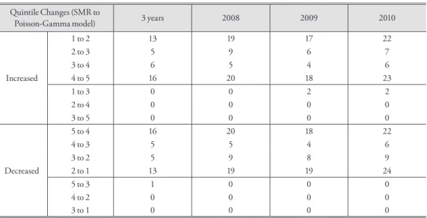
Table 3 shows the specific quantities of quintile change and the number of the region. The number of regions of positive and negative changes of quintile class is simi- lar. Whether the region has positive change or negative change of class, in most cases, it moves between 1-quin- tile and 2-quintiles or it moves between 4-quintiles and 5-quintiles. The regions where class change occurs toward the center have a relatively small birth count. On the other hand, the regions where class changes occur toward the 1 or 5-quintile range have a relatively large number of births.
In the 3 years’ aggregated data, Ongjin-gun, Jangsu- gun, Danyang-gun, Gurye-gun, and Muju-gun, moved from 1-quintile to 2-quintile after stabilization. In contrast, Guro-gu, Gwanak-gu, Yeongdeungpo-gu, Yongsan-gu, and Anseong-si moved from 2-quintile to 1-quintile. Seongdong-gu, Seocho-gu, Gangnam-gu, Seodaemun-gu, and Yeonsu-gu moved from 4-quintiles to 5-quintiles, and Ulleung-gun, Gunwi-gun, Cheon- gsong-gun, Yeongdeok-gun, and Bonghwa-gun moved from 5-quintiles to 4-quintiles. Yeongyang-gun moved from 5-quintiles to 3-quintiles, showing a 2-quintile change. In 2009, Gokseong-gun and Jangsu-gun showed 2-quintile class changes: 1-quintile to 3-quintiles. In
Table 2. The number of regions that changed their quintile classes
Statistics Years Quintile class changes
-2 -1 0 1 2
Difference of SMR and Poisson-Gamma model
3 years 0(0) 41(16.5) 168(67.5) 39(16) 1(0.4)
2008 0(0) 53(21.3) 143(57.4) 53(21.3) 0(0)
2009 2(0.8) 45(18.1) 153(61.4) 49(19.7) 0(0)
2010 2(0.8) 58(23.3) 128(51.4) 61(24.5) 0(0)
* The numbers in parentheses refer to percentages (%)
2010, Pyeongchang-gun and Ongjin-gun changed from 1-quintile to 3-quintiles. The regions shifted more than 2-quintile classes had a small LBW count or birth count.
By acceptance of the global mean, large change of quin- tile class have occurred in these regions because of the small sample size. In addition, their ranks of the LBW and birth counts placed in the 1st quintile.
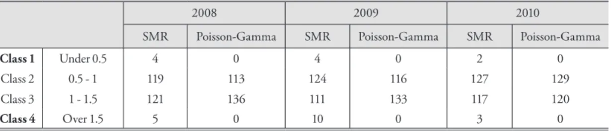
Table 4 summarizes the class frequencies of regions.
The classes were divided into four with equal intervals of 0.5. If a risk value was greater than 1.5, it was classified as Class 4. Therefore, Class 4 regions can be considered to have a relatively high risk of LBWs. On the other hand, if the RR was smaller than 0.5, the region was classified as Class 1 (i.e., regions with a low relative risk of LBW).
Some areas classified according to SMR values fell into Class 1 and 4. However, no regions were allocated to Class 1 or Class 4 when classifying regions with stabi- lized SMR. The regions assigned to Class 1 or 4 accord- ing to SMR had a small population and relatively low number of births. Due to the small number of popula- tion, the variability of SMR was relatively large. The sta-
bilized SMR statistics were weighted based on the global mean of the populations, so there are no regions classified as Class 1 or 4.
In 2008, there was a large variation between SMRs and the full Bayes model in Uiseong-gun, Inje-gun, Yangyang-gun, Seongju-gun, and Boeun-gun. In 2009, Cheongdo-gun, Hapcheon-gun, Yanggu-gun, Yeongyang-gun, and Jinan-gun showed large differences between before and after stabilization. In addition, there was a large difference before and after stabilization in Namhae-gun, Ulleung-gun, Jung-gu (Busan), Yeong- yang-gun, Yanggu-gun in 2010 and in Ulleung-gun, Yanggu-gun, Hapcheon-gun, Jung-gu (Busan), Jinan- gun in the 3 year aggregated data. In most cases, large difference values between SMR and shrink value are ob- served in the regions where the population is small (i.e., a low birth rate). In general, the smaller the population, the larger the shrinkage. The comparison shows that the higher RR shrunk much more toward the overall mean in rural than in urban regions.
Table 3. Counts of the areas with increased and decreased quintile classes Quintile Changes (SMR to
Poisson-Gamma model) 3 years 2008 2009 2010
Increased
1 to 2 13 19 17 22
2 to 3 5 9 6 7
3 to 4 6 5 4 6
4 to 5 16 20 18 23
1 to 3 0 0 2 2
2 to 4 0 0 0 0
3 to 5 0 0 0 0
Decreased
5 to 4 16 20 18 22
4 to 3 5 5 4 6
3 to 2 5 9 8 9
2 to 1 13 19 19 24
5 to 3 1 0 0 0
4 to 2 0 0 0 0
3 to 1 0 0 0 0
* Except for no changes
Figure 6. Mapping the differences of quintile classes based on the SMR and Bayes estimates ((a) 3 years aggregated data: (1a) SMR quintile map, (2a) quintile map of Poisson-Gamma model, (3a) Difference map,
(b) 2008: (1b) SMR quintile map, (2b) quintile map of Poisson-Gamma model, (3b) Difference map)
4. Discussion
Mapping is an effective way to visualize counts or rates of health data. We can provide easy and interesting health contents when we make a map using the preva- lence or mortality data in each unit area. The representa- tion of epidemiological data using maps and subsequent analysis of maps are commonly used in the analysis of health statistics and spatio-temporal patterns. Area- specific estimates of risk can give suggestions on public health resource allocations by estimating the disease bur- den in specific areas. In addition, as in the John Snow’s cholera maps, creating risk maps can be a clue to solve the hypotheses associated with health.
In this study, we produced prevalence maps of LBW in South Korea for the first time. SMRs are widely used to explain RRs in epidemiological fields. However, epide- miological maps and geographic visualization based on SMRs may give misleading of data due to a small number of cases or small populations in the study areas. There- fore, we used Bayesian models to calculate and depict sta- tistically reliable risk estimates of LBW in South Korea.
We used both empirical Bayes and full Bayes approaches for smoothing purposes. In addition, we compared maps of the posterior distribution of prevalence and the SMR.
We used the Poisson-Gamma model and full Bayesian methods. A Bayesian approach is warranted to accom- modate the posterior means in epidemiological mapping studies. The use of the Bayesian model provided more
reliable estimates of RRs in small areas. To compare the variability and range of the statistics computed by each method, we calculated the difference between SMRs and model-based estimates. We visualized SMRs, model- based estimates, and differences between the two meth- ods. The SMR method was the least efficient estimate of RRs. Bayesian approaches could be used to explore an excessive and low risk area with statistically reliable risk values. In this study, the result statistics and the vari- ance of empirical and full Bayesian analysis were similar.
Therefore, when considering the principle of Occam’s Razor, it would be more efficient to utilize the empirical Bayesian analysis.
The significance of this research study is that it high- lights the need for disease mapping and the current status of LBW in South Korea. In addition, this research provides statistically reliable risk maps of LBW in South Korea for the first time. LBW maps can be used for detec- tion of the areas that need to support medical assistance.
The limitation of this research is that it focused on cre- ating LBW prevalence maps. Therefore, this research did not include the statistical grouping or clustering of homogeneous high or low risk regions. Future research should be conducted to identify clusters of high- or low- risk regions of LBW prevalence in South Korea.
Table 4. Classification of the regions according to the relative risk classes of LBW
2008 2009 2010
SMR Poisson-Gamma SMR Poisson-Gamma SMR Poisson-Gamma
Class 1 Under 0.5 4 0 4 0 2 0
Class 2 0.5 - 1 119 113 124 116 127 129
Class 3 1 - 1.5 121 136 111 133 117 120
Class 4 Over 1.5 5 0 10 0 3 0
References
통계청, 2015, 2015 통계로 보는 여성의 삶.
Berkowitz, G.S., Skovron, M.L., Lapinski, P.H. and Berkow- itz, R.L., 1990, Delayed childbearing and the outcome of pregnancy, The New England Journal of Medicine, 322, 659-664.
Bernardinelli, L. and Montomoli, C., 1992, Empirical Bayes versus fully Bayesian analysis of geographical varia- tion in disease risk, Statistics in Medicine, 11, 983- 1007.
Besag, J., York, J., and Mollie, A., 1991, Bayesian Image Res- toration, with Two Applications in Spatial Statistics, Annals of the Institute of Statistical Mathematics, 43, 1-59.
Bureau of Health Policy, Ministry of Health & Welfare, 2011, 2012 Family health service guide.
Carriquiry, L. and Pawlovich, P., 2004, From Empirical Bayes to Full Bayes: Methods for Analyzing Traffic Safety Data, Iowa Library Services, URI: http://publica- tions.iowa.gov/id/eprint/13273.
Chomitz, V.R., Cheung, L.W.Y. and Lieberman, E., 1995, The role of lifestyle in preventing low birth weight, The Future of Children, 5(1), 121-138.
Clayton, D.G. and Kaldor, J., 1987, Empirical Bayes esti- mates of age-standardized relative risks for use in disease mapping, Biometrics, 43(3), 671-681.
Clayton, D.G.,1989, A Monte Carlo Method for Bayesian Infer- ence in Frailty Models, University of Leicester De- partment of Community Health Technical Report, Leicester, U.K.
Costello, J., Ortmeyer, C.E. and Morgan, W.K.C., 1974, Mortality from lung cancer in U.S. coal miners, American Journal of Public Health, 64(3), 222-224.
Elsen, E.A., Tolbert, P.E., Monson, R.R. and Smith, T.J., 1992, Mortality studies of machining fluid exposure in the automobile industry I: A standardized mor- tality ratio analysis, American Journal of Industrial Medicine, 22, 809-824.
Geronimus, A.T., 1996, Black/white differences in the rela- tionship of maternal age to birthweight: A popula- tion-based test of the weathering hypothesis, Social
Science & Medicine, 42(4), 589-597.
Kennedy, 1989, The small number problem and the accuracy of spatial databases, in Goodchild, M.F. and Gopal, S.
eds., Accuracy of Spatial Databases, Taylor & Francis, U.K., London.
Lawson, A.B., 2006, Statistical Methods in Spatial Epidemiol- ogy, 2nd ed., John Wiley & Sons Inc, UK.
Lawson, A.B., Biggeri, A.B., Böhning, D., Lesaffre, E., Viel, J.F., Clark, A., Schlattmann, P. and Divino, F., 2000, Disease mapping models: an empirical evalu- ation, Statistics in Medicine, 19, 2217-2241.
Lawson, A.B., Böhning, D., Biggeri, A., Lesaffre, E. and Viel, J.F., 1999, Disease mapping and its uses, in Lawson, A.B., Böhning, D., Biggeri, A., Lesaffre, E. and Viel, J.F. and Bertollini, R. eds., Disease mapping and risk assessment for public health, West Sussex, John Wiley
& Sons, U.K.
Lewis, G.H. and Johnson, R.G., 1971, Kendall’s Coefficient of Concordance for sociometric rankings with self- excluded, Sociometry, 34, 469-503.
Marshall, R.J., 1991, Mapping disease and mortality rates using empirical Bayes estimators, Applied Statistics, 40(2), 283-294.
Meliker, J.R., Wahl, R.L., Cameron, L.L. and Nriagu, J.O., 2007, Arsenic in drinking water and cerebrovascular disease, diabetes mellitus, and kidney disease in Michigan: a standardized mortality ratio analysis, Environmental Health, 6(4), 1-11.
Mollié, A. and Richardson, S., 1991, Empirical Bayes esti- mates of cancer mortality rates using spatial models, Statistical in Medicine, 10, 95-112.
Mollié, A., 1999, Bayesian and empirical Bayes approaches to disease mapping, In Disease Mapping and Risk Assess- ment for Public Health, Lawson, A.B., Biggeri, A., Boehning D, Lesaffre E, Viel, J-F., Bertollini, R.
(eds), Wiley, New York, 15-29.
Persaud, B., Lan, B., Lyon, C. and Bhim, R., 2010, Compari- son of empirical Bayes and full Bayes approaches for before-after road safety evaluations, Accident Analy- sis and Prevention, 42, 38-43.
Pickle, L.W. and White, A.A., 1995, Effects of the choice of age-adjustment method on maps of death rates, Sta-
tistics in Medicine, 14, 615-627.
Richardson, S., Thomson, A., Best, N. and Elliott, P., 2004, Interpreting posterior relative risk estimates in disease-mapping studies, Environmental Health Per- spectives, 112(9), 1016-1025.
Rush, D. and Cassano, P., 1983, Relationship of cigarette smoking and social class to birth weight and peri- natal mortality among all births in Britain, 5-11 April 1970, Journal of Epidemiology and Community Health, 37, 249-255.
Shiono, P.H. and Behrman, R.E., 1995, Low birth weight:
analysis and recommendations, Future Child, 5(1), 4-18.
Song, S.H. and Choi, E.S., 1999, Clinical Observation on Delivery of Low Birth Weight Infant, Journal of Korean Academy of Women’s Health Nursing, 5(2), pp.169-178.
Symons, M.J. and Taulbee, J.D., 1980, Standardized mortal- ity ratio as approximation to relative risk, Institute of Statistics Mimeo Series No.1294.
Tobler, W., 1970, A computer movie simulating urban growth in the Detroit region, Economic Geography, 46(2), 234-240.
Valero De Bernabé, J., Soriano, T., Albaladejo, R., Juarranz,
M., Calle, M.E., Martínez, D. and Domínguez- Rojas, V., 2004, Risk factors for low birth weight: a review, European Journal of Obstetrics & Gynecology and Reproductive Biology, 116, 3-15.
World Health Organization, 1950, Expert Group on Prematu- rity. Final report. Technical report series 27, World Health Organization, Geneva.
Ylppö A., 1919, Zur physiologie, klinik, zum schicksal der frühgeborenen, Zeitschrift für kinderheilkunde, 24, 1-110.
Young-hee Roh and Key-ho Park, 2014, A Comparative Analysis of SMR vs. Bayesian Modeling for Calcu- lating Statistically Reliable Relative Risks and Dis- ease Mapping, 한국지도학회지, 14(2), 107-117.
교신: 박기호, 08826, 서울시 관악구 관악로 1, 서울대학 교 지리학과(이메일: [email protected])
Correspondence: Key-ho Park, Department of Geography, Seoul National University, 1 Gwanak-ro, Gwanak-gu, Seoul, South Korea, 08826 (e-mail: [email protected])
Recieved March 14, 2016 Revised March 31, 2016 Accepted April 6, 2016