http://dx.doi.org/10.5369/JSST.2019.28.4.216 pISSN 1225-5475/eISSN 2093-7563
A Finite Memory Filter for Discrete-Time Stochastic Linear Delay Systems
Il Young Song+, Jin Mo Song, Woong Ji Jeong, and Myoung Sool Gong
Abstract
In this paper, we propose a finite memory filter (estimator) for discrete-time stochastic linear systems with delays in state and mea- surement. A novel filtering algorithm is designed based on finite memory strategies, to achieve high estimation accuracy and stability under parametric uncertainties. The new finite memory filter uses a set of recent observations with appropriately chosen initial horizon conditions. The key contribution is the derivation of Lyapunov-like equations for finite memory mean and covariance of system state with an arbitrary number of time delays. A numerical example demonstrates that the proposed algorithm is more robust and accurate than the Kalman filter against dynamic model uncertainties
Keywords: Data Fusion, Time Delay, Finite Memory
1. INTRODUCTION
The problem of state estimation for dynamic systems with time delays has received a great deal of research interest. The time delay phenomenon in state variables is unavoidable in many real systems [1]. For example, LEO satellite communication systems have multiple channel delays [2]. Hence, remote control of robot systems can be conducted in a cloud platform through data connection with a robot manipulator. The important applications of cloud robotics can be found in space exploration, remote surgery, intelligent housing systems, unmanned vehicles, and so on [3]-[7]. These systems have motivated researchers to study the control and filtering problem of systems with time delays [8].
Using finite-memory estimation, we can obtain an estimate based on data from the recent past only (finite memory). As a result, finite memory Kalman filters are more robust against model uncertainties and numerical errors than standard Kalman filters, which utilize all measurements [9, 10]. Thus, a finite memory filter was chosen in this study.
Based on the aforementioned literature, and to the best of the authors’ knowledge, there are no existing results for finite
memory filtering for linear systems with time delays. Motivated by the above problems, we focus on estimating the state of a discrete-time linear system with time delays in both the state and observation matrices, using a finite memory strategy. We derive from crucial Lyapunov-like equations, finite memory mean and covariance of systems with an arbitrary number of time delays.
Moreover, the obtained results are valid for general linear systems with time delays in both dynamic and observation models.
The remainder of this paper is organized as follows. In Section II, the problem statement is given. In Section III, we present the finite memory filter for discrete-time linear systems with time delays. Here, the exact and recursive equations for determining the finite memory initial conditions (mean and covariance) are derived and discussed. In Section IV, an implementation of a stochastic system with uncertainties is considered to compare between the Kalman filter with time delays (KFTD) and the proposed finite memory filter. The effectiveness and comparative analysis of the proposed filter with the KFTD are then presented.
Finally, we provide a summary of our conclusions in Section V.
2. PROBLEM STATEMENT
We first consider a discrete-time linear system described by stochastic recursive equations with time delays:
(1)
where is an unknown state, , h=0,1,…,M are
time-varying matrices, , are
( ) M h( ) ( ) ( )
h 0
x k 1 F k h x k h w k , k 0,1,...,
=
+ =∑ − − + =
( ) n
x k ∈ℜ F kh( )
n n× x s ~ x ,P( ) (− Ν 0 0) s 0,1,...,M=
Department of Sensor Systems, Hanwha Corporation Defense R&D Center, 305 Pangyo-ro, Bundang-gu, Seongnam-si, 13488, Korea
+Corresponding author: [email protected] (Received : Jul. 15, 2019, Accepted : Jul. 30, 2019)
This is an Open Access article distributed under the terms of the Creative Commons Attribution Non-Commercial License(http://creativecommons.org/
licenses/bync/3.0) which permits unrestricted non-commercial use, distribution, and reproduction in any medium, provided the original work is properly cited.
initial conditions, is a zero-mean white Gaussian
noise with covariance , and is the
Kronecker function.
The discrete measurement is:
(2)
where , d=0,1,…,L is the measurement matrix, and is a zero-mean white Gaussian noise with covariance
.
We also assume that the initial states: , s=0,1,…,M, system noise , and measurement errors are mutually uncorrelated, i.e.,
(3)
The main problem associated with such a system is then to find the estimate of the unknown state x(k) based on the overall horizon sensor measurement y(k) with horizon time intervals i.e.,
(4) Using KFTD’s equations for the system (1) and (2) presented by Mishra [11] and Priemer [12], we propose their finite memory version for estimation of state x(k) using finite memory measurements y(k) in (4). The details of our new Finite Memory Kalman Filter with Time Delays (FMKFTD) are described in the next section.
3. A FINITE MEMORY FILTER FOR SYSTEMS WITH TIME-DELAYS
The KFTD’s equations for the system (1) and (2) presented by [11] and [12] are used to find based on finite memory measurements y(k), we obtain:
(5)
(6)
(7)
where the finite memory filter gains and error auto-covariances
(8) are described as follows by:
(9)
(10)
(11) In contrast to the KFTD filtering, the finite memory filtering (5)-(11) needs to initialize (M+1) horizon initial conditions at which represents an unconditional means and covariance, i.e.,
(12) And
(13) Theorem 1: The horizon initial means (12) are described by
(14)
with initial conditions:
(15) Theorem 2: The horizon initial covariances (13) satisfy Lyapunov-like recursive equations
(16)
( ) n
w k ∈ℜ
( ) ( )
{ } ( ) ks
cov w k ,w s =Q k δ δks
( ) m
y k ∈ℜ
( ) L d( ) ( ) ( ) ( ) m
y k d 0H k d x k d v k , y k ,
=
=∑ − − + ∈ℜ
( ) m n
H kd ∈ℜ×
( ) m
v k ∈ℜ
( ) ( )
{ } ( ) ks
cov v k ,v s =R k δ
( )
x s−
( )
w k v k( )
( ) ( )
{ } { ( ) ( )}
( ) ( )
{ }
cov x s , w k 0, cov x s ,v k 0, cov w k ,v k 0, s 0,1,...,M.
− = − =
= =
, Δ
{ }
y(k)= y(s): s=k-Δ,k-Δ+1,...,k .
( )
ˆx k|k
( ) ( )
( ) ( ) ( ) ( )
{ }
0
ˆ ˆ 1
ˆ 1
1 1,2,...,M M
L
m d=
x s - m | s = x s - m | s -
+G s y s - H s - d x s - d | s - , s = k - , k - + , ..., k ,
m = , = max M,L .
⎡ ⎤
⎢ ⎥
⎣ ⎦
Δ Δ
∑
( ) ( ) ( )
0
ˆ 1 M 1 ˆ 1 1
h=
x s | s - =∑F s - h - x s - h - | s - .
( ) ( ) 0( ) ( ) ( ) ( )
0
ˆ ˆ 1 L ˆ 1
d=
x s|s =x s|s- +G s y s -⎡ H s-d x s-d|s- ⎤.
⎢ ⎥
⎣ ∑ ⎦
( )
m k
G , m = ,0 1,2,...,M
( ) { ( ) ( )}
( ) ( ) ( )
1 2 1 2
1 1 1 2
cov ˆ
P s ,s |s = e s |s ,e s |s , e s |s =x s -x s |s , s ,s s.≤
( ) ( ) ( )
( ) ( ) ( ) ( )
1 2
0
1
1 1 2 2
0
1
1
L T
m d=
L -
T d ,d =
G s = P s - m,s - d | s - H s - d
R s + H s - d P s - d ,s - d | s - H s - d .
⎡ ⎤
×⎢ ⎥
⎣ ⎦
∑
∑
( ) ( )
( ) ( ) ( )
1
1 2 1 2
0 2
1
L 1
h d=
P s - h ,s - h | s = P s - h ,s - h | s -
-G s ∑H s - d P s - d,s - h | s - ,
( ) ( ) ( ) ( ) ( )
1 2
1 1 2
0
1 1 M E T
h ,h =
P s+ ,s+ |s =∑F s-h P s-h,s-h |s F s-h + Q s .
s=k-Δ
( ) { ( )} ( )
( ) { ( )} ( )
( ) { ( )} ( )
ˆ - - 1 - - - 1 - - 1 ,
ˆ - - 2 - - - 2 - - 2 ,
...
ˆ - 1 - - 1 - 1 .
x k M k E x k M m k M
x k M k E x k M m k M
x k k E x k m k
Δ + Δ = Δ + ≡ Δ +
Δ + Δ = Δ + ≡ Δ +
Δ+ Δ = Δ+ ≡ Δ+
( 1 2 ) { ( ) ( )1 2} ( 1 2)
1 2
, - cov , , ,
, - - 1, ..., - 1
P h h k x h x h P h h
h h k M k
Δ = ≡
= Δ + Δ+
( ) ( ) ( )
0
1 M ,t 0,1,2,...,k,k 1
h=
m t+ = F t -h m t -h =∑ −Δ+
( ) ( ) ( )0 1 2 ... ( )M x .0
m = m − =m − = = −m =
( ) ( ) ( ) ( )
( )
1 2
1 1 2 2
0
1 1
0,1, 2, ..., 1,
M T
h ,h =
P t + ,t + = F t - h P t - h ,t - h F t - h + Q t , t = k - +Δ
∑
(17)
with initial conditions:
(18) Derivation of Lyapunov-like equations for mean and covariance (14)-(18) is included in the appendix.
Remark. Original initial conditions for the KFTD at different time instants are identical in contrast to horizon initial conditions (12) and (13) that more realistically.
4. NUMERICAL EXAMPLE
In this section, we present an example for discrete-time dynamic systems with parametric model uncertainty . The example demonstrates the robustness of the proposed FMKFTD (5)-(18) in terms of mean square errors (MSEs).
We now consider the following LEO satellite communication system with multiple time delay and uncertainty [2]. Low earth orbit satellite channels impart severe spreading in delay and oppler on the transmitted signal. The state vector x represents the received signal level [dB]:
(19)
where is a white Gaussian noise. The system noise intensity is and the measurement noises are also zero- mean white Gaussian noises with covariances The
initial values are [dB] and
These are uncertain model parameters which are assumed to satisfy
(20)
where is the uncertainty interval (UI). The horizon
length Δ of the FMKFTD is taken as ,
respectively. The FMKFTD and KFTD (non-finite memory version with time delays) [6, 7] for the system model (19) with the uncertainty which takes the form (20) are compared.
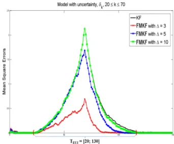
We now present model (19) to show the robustness of the finite
memory filter against the uncertainty . All simulations were evaluated in terms of the MSEs of 1000 Monte Carlo runs. Fig. 1 compares the MSEs of FMKFTD (“FMKF”) with three KFTDs (“KF”) with three different finite memory lengths Δ,
(21)
Owing to the fact that the uncertainty has little effect on the behavior of the filters (estimates) after the extremity of interval , for convenience of MSE analysis we introduce the extended time interval , referred to as the Extended Uncertainty Interval (EUI). According to the simulation results, and , our point of interest is the behavior of the aforementioned filters, both inside and outside of the time-interval .
As shown in Fig. 1, we can observe that inside the EUI, FMKFTD demonstrates good performance when compared to KFTD; this is in general agreement with the robustness of the finite memory strategy. The MSEs of the non-finite memory filter KFTD is notably larger than the FMKFTD. However, the KFTD performs slightly worse than the FMKFTD with a horizon length of . Also, the FMKFTD with the horizon length is more accurate than the FMKFTD with horizon lengths and
, such that:
(22) The reason for the presence of such a robust property (22) is to compensate for the given uncertainty , as the horizon length
( ) ( ) ( )
( )
( ) ( )
1
1 2 1 1 1 1 2
0
1 T
1 2 2 1
1 1 1
,
, ,
1 2
M l =
t-h ,t-h 1 2
1 2
P t - h + ,t - h + = F t - h -l P t - h -l ,t - h + Q t - h , k - h k - h P t - h ,t - h P t - h ,t - h t - h t - h
δ
+
≥
= <
∑
( 1 2) 0, ,1 2 0,1, 2, ..., M P -s ,-s = P s s = .
0,-1, -2, ..., -M s =
( )k
δ
( ) ( ) ( ) ( ) ( )
( ) ( ) ( )
( ) ( ) ( ) ( ) ( )
1 2
3
1 0.995 0.190 1
0.107 2
0.4 0.1 1 0.4 2
x k+ = +δ x k + +δ x k -
+ +δ x k - +w k ,
y k = x k + x k - + x k - +v k .
⎧⎪
⎨⎪
⎩
( )
w k
( )
Q k 0.022 v k( )
R k( ) 0.5=
( )0 ~ N( ( ) ( )0 , 0 ,) ( )0 1=
x x P x
( )0 =1.
P δ( )k
( )k δ1 0.05,δ2 0.1,0, δ3 0.01, otherwisek TUI,,
δ = ⎨⎧⎪ ≤ ≤ ≤ ∈
⎪⎩
[20; 70]
UI = T
3, 5, and 10 Δ =
( )k
δ
( )k
δ
( ) ( ) ( ) ( ) ( ) ( )
2 2
ˆ ,
and ˆ , 3,5,10.
KF KF
FMKF KF
P k k E x k x k k
P k k E x k x k k
⎡ ⎤
= ⎣ − ⎦
⎡ ⎤
= ⎣ − ⎦ Δ =
( )k
δ
k = 70
20; 70 ε
=⎡⎣ + ⎤⎦ TEUI
ε=60 TEUI= ⎡⎣20; 130⎤⎦
20; 130
= ⎡⎣ ⎤⎦ TEUI
10
Δ = Δ =3
5 Δ = 10
Δ =
( 3) ( 5) ( 10) , .
FMKF FMKF FMKF KF
k k k k EUI
P Δ = <P Δ = <P Δ = ≈P k T∈
( )k
δ
Fig. 1. MSEs comparison between KFTD and three FMKFTD
Δ for sensors (memory of FMKFTD) should be minimal. In this case .
Here, we observe that the MSEs of the non-finite memory filter KFTD is remarkably large in contrast to the finite memory version FMKFTD. This means that for our example the application of the FMKFTD can produce good results in real-time processing requirements.
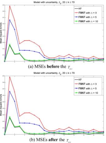
On the other hand, Fig. 2 shows that outside the TEUI the KFTD is better than all FMKFTD, i.e.,
(23) It should also be noted that the reduction of the horizon length to zero inside the uncertainty interval is impossible due to the loss of sensor measurements (23). Thus, the problem in finding the optimal horizon length Δ for each individual FMKFTD is quite complex.
5. CONCLUSIONS
In this paper, we propose a new finite memory filter for discrete-time linear systems with uncertainties and time delays in
both the state and observation matrices. Simulation analysis and comparison with the KFTD verifies the effectiveness of the proposed solution, FMKFTD. FMKFTD can be widely used in many practical applications. The Lyapunov-like equations for finite memory mean and covariance of system state with an arbitrary number of time delays are derived.
REFERENCES
[1] B. D. O. Anderson and J. B. Moore, Optimal Filtering, Prentice-Hall, City, 1979.
[2] S. C. Burleigh, T. D. Cola, S. Morosi, S. Jayousi, E. Cianca, and C. Fuchs, “From Connectivity to Advanced Internet Services: A Comprehensive Review of Small Satellites Communications and Networks”, Wireless Commun Mob.
Comput., Vol. 2019, pp. 6243505(1)- 6243505(17), 2019.
[3] S. Al-Wais, R. Mohajerpoor, L. Shanmugam, H. Abdi, and S. Nahavandi, “Improved delay-dependent stability criteria for telerobotic systems with time-varying delays”, IEEE Trans. Syst. Man Cybern. Syst. Vol. 48, No. 12, pp. 2470 2484, 2017.
[4] K. Sugiura, Y. Shiga, H. Kawai, and T. Misu, “A cloud robotics approach towards dialogue-oriented robot speech”, Adv. Robot., Vol. 29, pp. 449 456, 2015.
[5] H. Jahanshahi, M. Jafarzadeh, N.N. Sari, V. T. Pham, V. V.
Huynh, and X. Q. Nguyen, “Robot motion planning in an unknown environment with danger space”, Electronics, Vol.
8, No. 2, pp. 201-228, 2019.
[6] L. Ding, Q. L. Han, and X. Zhang, “Distributed secondary control for active power sharing and frequency regulation in islanded microgrids using an event-triggered communica- tion mechanism”, IEEE Trans. Ind. Inform., Vol. 15, No. 2, pp. 3910-3922, 2019.
[7] M. Rabah, A. Rohan, Y. J. Han, and S. H. Kim, “Design of fuzzy-PID controller for quadcopter trajectory-tracking”, Int. J. Fuzzy Log. Intell. Syst., Vol. 18, pp. 204 213, 2018.
[8] M. M. Zavarei and M. Jamshidi, Time-Delay Systems: Anal- ysis, Optimization and Application, North-Holland, Amster- dam, 1987.
[9] D. Y. Kim and V. Shin, “Optimal receding horizon filter for continuous-time nonlinear stochastic systems”, Proc. 6th WSEAS Inter. Conf. on Signal Process., Dallas, Texas, USA, pp. 112 116, Mar 2007.
[10] D. Y. Kim and V. Shin, “An optimal receding horizon FIR filter for continuous-time linear systems”, Proc. Intern.
Conf. SICE-ICCAS, Busan, Korea, pp. 263 265, Oct 2006.
[11] J. Mishra and V. S. Rajamani, “Least-squares state esti- mation in timedelay systems with colored observation noise: an innovation approach”, IEEE Trans. Automat.
Contr., Vol. 20, No. 1, pp. 140 142, 1975.
[12] R. Priemer and A. G. Vacroux, “Estimation in linear dis- cretesystems with multiple time delays”, IEEE Trans.
Automat. Contr., Vol. 14, No. 4, pp. 384 387, 1969.
3 Δ =
( 10) ( 5) ( 3 ,) .
KF FMKF FMKF FMKF
k k k k EUI
P <P Δ = <P Δ = <P Δ= k T∉
(Δ →0)
Fig. 2. MSEs comparison between three FMKFTD and KFTD out- side the TEUI
APPENDIX
Derivation of the equation for horizon initial mean (14) Taking expectations on both sides of (1) and using , we immediately obtain the recursive equation (14) for mean
.
Derivation of the equation for finite memory initial covariance (16)
Subtracting (14) from (1) we obtain time propagation of the centered state as follows:
(A.1)
Next we have:
(A.2)
Taking expectations on both sides of (A.2) and using the fact that current noise does not depend on current and past states ,we obtain the recursive equation for covariance (16):
(A.3) Note that equation (A.3) contains auto-covariance:
(A.4)
Derivation of the equation for auto-covariance (17) Using the “symmetric” property of auto-covariance
and without loss of generality we can assume that . Substituting in (A.1) we obtain:
(A.5) Multiplying both sides of (A.5) by and using (A.4) we obtain:
(A.6)
and
(A.7) We then calculate the expectation in (A.7), i.e.,
(A.8) We calculate the product using (A.5) and after taking that expectation, we get:
(A.9)
According to assumption , “future” noise does not depend on current and past states
therefore
Next using the property of white noise we obtain:
(A.10)
Finally using (A.7), (A.9) and (A.10) we get the equation for auto-covariance (17). This completes the derivation Lyapunov- like equations for finite memory mean and covariances.
( ) 0
E w t⎡⎣ ⎤ =⎦
( ) [ ]( )
m t =E x t
( ) ( ) ( ) ( )
0
1 M h - - , 0,1, 2,...,
h
x t F t h x t h w t t
=
+ =∑ + =
% %
( ) ( ) ( ) ( ) ( ) ( )
( ) ( ) ( ) ( ) ( ) ( ) ( ) ( )
12
1
2
1 1 2 2
, 0
1 1
0
2 2
0
1 1 - - - -
- -
- - .
T M T T
h h
T M T
h
M T T
h
x t x t F t h x t h x t h F t h
w t w t F t h x t h w t
w t x t h F t h
=
=
=
+ + =
+ +
+
∑
∑
∑
% % % %
%
%
( )
w t
( - 1), ( - 2)
x t h% x t h%
( ) ( ) ( ) ( ) ( )
1 2
1 1 2 2
, 0
1, 1 M - - , - T - .
h h
P t t F t h P t h t h F t h Q t
=
+ + = ∑ +
( ) ( ) ( )
( ) ( ) ( )
1 2 1 2
1 2
- , - - - ,
- - - - ,
, 0,1,..., .
P t h t h E x t h x t h T
x t h x t h m t h
h h M
=
=
=
⎡ ⎤
⎣% % ⎦
%
( - , -2 1)
P t h t h =
( - , -1 2)T
P t h t h
1 2
- -
k h ≥k h t→t h- 1
( ) ( ) ( ) ( )
1
1 1 1 1 1 1
0
- 1 M - - - - - .
l
x t h F t h l x t h l w t h
=
+ =∑ +
% %
( - 2 1)T
x t h +%
( ) ( ) ( ) ( ) ( )
( ) ( )
1
T T
1 2 1 1 1 1 2
0
T
1 2
- 1 - 1 = - - - - - 1
- - 1 ,
M l
x t h x t h F t h l x t h l x t h
w t h x t h
=
+ + +
+ +
∑
% % % %
%
( ) ( ) ( )
( ) ( )
1
1 2 1 1 1 1 2
0
T
1 2
1 2
- 1, - 1 - - - - , - 1
- - 1 ,
, 0,1,..., .
M
l
P t h t h F t h l P t h l t h
E w t h x t h
h h M
=
+ + = +
+ +
=
⎡ ⎤
⎣ ⎦
∑
%
( - 1) ( - 2 1)T - 1 - 2
E w t h x t h⎡⎣ % + ⎤⎦ for t h t h≥
( - 1) ( - 2 1)T
w t h x t h +%
( ) ( ) ( ) ( ) ( )
( ) ( )
2
T T T
1 2 1 2 2 2 2
0
T
1 2
- - 1 - - - - -
- - .
M l
E w t h x t h E w t h x t h l F t h l
E w t h w t h
=
+ =
+
⎡ ⎤ ⎡ ⎤
⎣ ⎦ ⎣ ⎦
⎡ ⎤
⎣ ⎦
∑
% %
1 2
- -
t h ≥t h
( - 1)
w t h
( - -2 2)
x t h l% E w t h x t h l⎡⎣ ( - 1) (% - -2 2)T⎤⎦=0.
( - 1) ( - 2)T ( - 1) t h t h- , -1 2. E w t h w t h⎡⎣ ⎤⎦=Q t h δ