Characteristics of tidal turbulence near the bottom at a coastal trench in Tongyoung, Korea

J Kor Soc Fish Technol, 50 (4), 435―446, 2014 http://dx.doi.org/10.3796/KSFT.2014.50.4.435

<Original Article>

Characteristics of tidal turbulence near the bottom at a coastal trench in Tongyoung, Korea

Yonghae KIM^*, Chul-Hoon HONG¹

Institute of Marine Industry, College of Marine Science, Gyeongsang National University, Tongyeong, 650-160, Republic of Korea

1Div. of Marine Production System Management, Pukyong National University, Busan, 608-737, Republic of Korea

Tidal turbulence was examined using three-dimensional tidal velocity data observed at a trench offshore of Tongyoung, Korea. The kinetic energy and intensity, including the variation period of the flow velocity and direction, were used to investigate the relationships between tidal turbulence and fishing gear dynamics, including the effects of swimming fish during fishing operations. As the resultant velocity increased from 0.2 to 0.9 m/s, the kinetic energy also significantly increased, while the turbulence intensity decreased from 50 to 10%. Tidal flow in strong flow fields displayed shorter periods of between 4 and 10 s, as determined by fast Fourier transform, the global wavelet method, and peak event analysis, and the periods were compared with the period of response to swimming fish and to oscillation of fishing gear. As mean velocity increased, velocity amplitude also increased from 0.1 to 0.6 m/s, and its directional amplitude changed markedly from 20 and 90°. Our study suggests that tidal turbulence can influence fish behavior or fishing gear geometry during fishing operations, although our analysis considered only a limited area. In future work, observations should be carried out over a more extensive depth and area.

Keywords: Tidal flow, Kinetic energy, Turbulence intensity, Period and amplitude

*Corresponding author: [email protected], Tel: 82-55-772-9183, Fax: 82-55-772-9189

Introduction

Turbulence in tidal currents affects on the movement of animals and fishing gear operations. Recently, the turbulence flow as a three-dimensional (3-D) component of velocity was measured in coastal tides and analyzed using acoustic Doppler current profilers (ADCP) or acoustic Doppler velocimeters (ADV) (Thorpe, 2007).

The turbulence flow, which can be defined by the velocity field, is not repeatable in either the whole or part of the flow domain referred to as laminar flow (Bernard and Wallace, 2002). In nature, water is generally in a state of non-uniform and variable motion that is referred to as “turbulence”, al-

though there exists no straightforward, unambiguous defi- nition of the term (Thrope, 2007). Turbulence is generally accepted to be an energetic, rotational and eddying state of motion that results in the dispersion of material and the trans- fer of momentum, heat and solutes at rates far higher than those of molecular processes alone.

Turbulence is often dominated by coherent structure activ- ities and turbulent events which may be defined as a series of turbulent fluctuations that contain more kinetic energy than the average turbulent fluctuations within the relevant section.

Therefore, studies in tidal areas of 3-D turbulence structures

have been hampered by the limited size of the observed area

due to equipment limitations; e.g., Laser Doppler Velocimetry in tank experiments (Pichot et al., 2009).

The characteristics of turbulence in tidal flow have been investigated in various contexts, such as sediment suspension (Ham et al., 2001; Chanson, 2010; Chanson et al., 2011; Yuan et al., 2009 ), tidal straining (Simpson et al., 2005; Thorpe et al., 2008), and tidal energy turbines (Rippeth et al., 2003;

Thomson et al., 2012).

Turbulent flow can affect swimming fish (Shadwick and Lauder, 2006; Liao, 2007; Webb and Cotel, 2010; Tritico and Cotel, 2010) and fish escape from codends (Kim, 2012;

2013a). Flow inside codends was analyzed by measuring the turbulence intensity and periodicity for shrimp beam trawls and bottom trawls (Kim, 2012; 2013a). Flow inside codend towed fishing gear may be affected primarily by tidal flow, followed by wakes inside fishing gear (Bouhoubeiny et al., 2011) and ship motion including the wave effect (O’Neill et al., 2003). Turbulence measurements close to Korea were car- ried out in the western Yellow Sea off the coast of China in both relatively shallow (Liu et al., 2009a; 2009b; Yuan et al., 2009) and deeper (Lozovastsky et al., 2012) waters.

Thus, the 3-D components of tidal turbulence can affect animal kinetics such as swimming performance, or the drag or wake of fishing gear. However, tidal turbulence at the sea bottom has, to our knowledge, not been analyzed in Korean waters as precise high-frequency 3-D flow. Hence, the pur- pose of this preliminary study was to determine the physical elements of tidal turbulence, such as turbulence intensity and dominant period focused on fish movement and fishing gear dynamics. Two locations at a trench between Manjido and Bujido offshore of Tongyoung, Korea were selected for their different geological conditions and as locations used as the fishing grounds for shrimp beam trawls, two-boat seine nets, etc. 3-D flow measurement data were collected using ADV and the kinetic energy, turbulence intensity, and period in re- lation to fishing gear dynamics and movements of swimming fish during fishing operations were analyzed.

Materials and methods

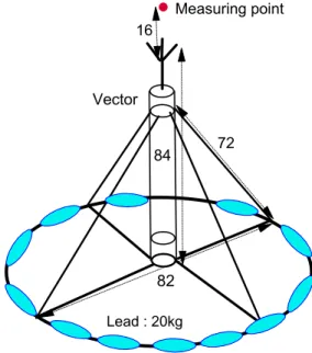
Tidal flow was measured using a three-component acoustic Doppler velocimeter (Vector, Nortek, Norway) as described in previous studies (Kim, 2012; 2013a). The velocimeter was

set in an upright position using a circular frame of 10-mm iron rods and 20-kg lead weights to anchor it firmly on the seabed (Fig. 1). The velocimeter measured water velocity based on a volume of water of 1.5-cm diameter 16 cm from the acoustic probe with an accuracy of ±0.5% according to the manufacturer’s specifications. The overall length of the velocimeter was 82.5 cm; its diameter was 7.5 cm; and its weight in water was 1.5 kg. The instrument also included sen- sors for measuring temperature (accuracy, 0.1°C), direction (compass accuracy, 2°), tilt (pitch and roll accuracy, 0.2°), and depth pressure (accuracy, 0.25%). A holding frame that formed a quadratic pyramid (diameter 82 cm, height 63 cm) was used to maintain the device in the orthogonal position, maintaining its sampling position at 1 m above the seabed.

The equipment was deployed with 8-mm PP rope of 1.5 times length of depth in connection with a 2.5 kg weight and a spherical buoy (diameter, 30 cm) to a upright rod with a flag on the surface.

Observations were performed at two sites at a deep trench between Manjido and Bujido south-west of Tongyoung, as shown in Fig. 2. The trench was oriented north-west to south-east at depths ranging between 50 and 70 m, while the depth of the surrounding area ranged between 30 and 40 m.

These sites are generally used as the primary fishing ground

84

Measuring point

Vector

Lead : 20kg 16

82

72

Fig. 1. Vector velocimeter set-up in the upright position with a circular frame (P: measuring position, units are cm).

of coastal fishing boats, including those using shrimp beam trawls and two-boat seine nets. Measurements were carried out five times (at sites S1, 2, 4, 5, 6) west of Manjido and once (site S3) north of Bujido. The sampling times and tidal conditions are shown in Table 1.

Tidal flow velocity was defined as three components: east (positive)-west (negative) velocity (V

), north (positive)-south (negative) velocity (V

), automatically designated by internal compass, and depth (V

) directions. Vector measurements of tidal current were set at 2 m/s maximum velocity as a 3-D axis with east, north and depth directions with a 16-Hz sam- pling rate mostly at 34 practical salinity units (psu). The acoustic speed was also calibrated automatically using data from the temperature and pressure sensors, and all sampling data were stored in internal memory.

Following data collection at sea, the landing state of the data was checked using the tilt, noise and correlation data.

When the standard deviation of the pitch or roll data per sec- ond was higher than the tilt accuracy; i.e., 0.2°, the vector could be shaking due to slack landing. Therefore, measure- ments taken at Stations S4 and S5 with a tilt of pitch and roll >1° were not included in the analysis (Parra et al., 2014).

Additionally, for the 3-D flow velocity data, average signal to noise ratios <15dB and average correlation values <70%

were eliminated (McLelland and Nicholas, 2000).

Based on the definition of turbulence flow in Bernard and Wallace (2002), the tidal turbulent flow was analyzed as tur- bulence intensity, kinetic energy and oscillation period for

analysis of the fisheries variables. The three components (V

,

, V

) of velocity data for the entire measurement period for each site were assessed every 1 min (data n=480 = 8 Hz × 60 s or 960 = 16 Hz × 60 s) to determine turbulence intensity and kinetic energy, as shown in Table 2. The mean resultant velocity U

represents an estimate for consecutive 1-min sam- ples as follows:

Tongyoung Mirukdo

Chudo 20m

50m S1,2,4,5,6

128 15'E 20' 25'

34 40'N

45' 50'

o o

50m

S3

Bujido Yondaedo

Yokjido

Manjido

Fig. 2. Map of observation sites (S1–6) at a trench offshore of Tongyoung, Korea.

Table 1. Sampling stations and tidal conditions

Station Lat. Long. Depth

(m)

Duration (start-end) (KST)

Sampling

rate (Hz) Tide day Time (range)*

(KST, cm)

S1 34° 44.2′N 128° 22.2′E 65 9:15-13:00, 27 Oct 2011 8 8 8:57(293) 14:55(27)

S2 34° 44.3′N 128° 22.1′E 65 13:58, 6 Apr- 16 8 14:22(-9) 20:54(274)

16:13, 7 Apr 2012 9 9:05(265) 15:00(-18)

S3 34° 42.9′N 128° 23.8′E 60 10:10-20:50, 3 Dec 2013 16 8 9:02(282) 15:02(35)

S4 34° 44.1′N 128° 22.2′E 65 10:00-14:30, 4 Nov 2013 16 9 9:12(280) 15:11(40)

S5 34° 44.1′N 128° 22.2′E 65 20:00, 16 Nov- 16 6 20:05(230)

06:37 17 Nov 2013 7 2:03(36) 8:32(262)

S6 34° 44.1′N 128° 22.2′E 68 20:50, 30 Mar- 16 7 20:57(267)

8:07, 31 Mar 2014 8 2:53(2) 8:55(260)

* High and low tide with tidal difference from tide table

Table 2. Sampling times of turbulence intensity measurements and periods of strong flow

Station

Total sampling Strong tide selection

Duration

(min) No. of

measurements Symbol Start time

(KST) Flow Duration

(min) No. of

measurement S1

S2

S3

S6

215 1,576

638

671

103,050 1,513,119

612,480

644,160

S1a S2a S2b S2c S2d S3a S3b S6a

9:31 17:17

5:15 7:26 0:57 12:52 18:15 4:00

Ebb Flood Flood Flood Ebb Ebb Flood Flood

53 18 27 13 17 83 47 38

25,600 16,820 25,800 12,200 15,600 80,401 45,000 36,100

Um

= (V

+ V

+V

)

(1)

Accordingly S

, S

, and S

represent the standard deviation of flow velocities per minutefor V

, V

, and V

, respectively.

Then, turbulence kinetic energy (K

, m

/s

)can be represented as:

Ke

= (S

+S

+S

) / 2 (2)

Next , the turbulence intensity (T

, %) as a ratio can be defined as the square root of K

divided by the mean flow velocity U

as:

Tr

= K

/ U

(3)

For periodic analysis, each sampling dataset recorded at 8 and 16 Hz was converted for each resultant velocity (Vr) and horizontal flow direction (Ab) using the V

and V

components for strong tides of six flood durations and two ebb durations during each measurement (Table 2). Using these converted data, the specific period was estimated by fast Fourier trans- form (FFT), global wavelet method, and Morlet wavelet method.

MATLAB (MathWorks) was used to analyze the perio- dicity of the tidal flow velocity and direction for shorter peri- ods <30 s using FFT for selected strong flood or ebb data from each measurement. The Morlet wavelet method in MATLAB was well localized in both time and space for pe- riodicity analysis, as applied in many studies (Yuan et al., 2009; Seena and Sung, 2011). The Morlet continuous wavelet method (CWT) was also viewed for 2000 burst sampling data for shorter periods <10s, which was more relevant for the analysis of swimming fish (Kim et al., 2008) or fishing gear

movements (O’Neill et al, 2003; Kim, 2012; 2013a). In addi- tion, the global and Morlet wavelet spectra for velocity and direction were calculated to determine the moderate dominant period <30 s using software from Torrence and Compo (1998) and Zhang et al. (2010).

The above methods, however, are unable to calculate the amplitude as the velocity or directional range of a period, and are also unsuitable for periodic data with a wide range.

Therefore, the event analysis method, such as the difference

between peak and valley values, was adapted using software

designed by ourselves based on Narasimha et al. (2007) to

analyze the depth change of the shaking codend (Kim,

2013b). When the depth increased until the peak and then

decreased in consecutive time series data, the peak value was

detected as a positive peak value, and the valley value was

detected as a negative valley value. Fig. 3 shows the results

using the event analysis method for Station S2b. The mini-

mum time interval between peaks or valleys was limited to

1 s, taking into consideration the sampling rate and oscillation

of fishing gear (O’Neill et al., 2003; Kim, 2013a). The initial

threshold value (Vi, +:peak, -:valley) between neighboring

peaks or neighboring valleys was categorized by the mean

value ± 0.5 SD for data at 30-s intervals, respectively. Then,

a peak event value (Vp+ for peak, Vp- for valley) can be

selected as the highest value among Vi. The mean period was

estimated from the average of the total intervals between

peaks and between valleys, while the mean amplitude was

estimated from the velocity or directional difference between

peak events and valley events that occurred only consec-

utively as a pair.

0 10 20 30 40 50 60 Time (s)

0.0 0.2 0.4 0.6 0.8 1.0 1.2

Resultant velocity (m/s)

Vr Vi+ Vi- Vp+ Vp-

(A)

(B)

0 10 20 30 40 50 60

Time (s) 240

270 300 330 360

Tidal direction (deg)

Ab Ai+ Ai- Ap+ Ap-

Fig. 3. Peak and valley events of the resultant velocity (A) and direction (B) from Station S2b.

V: velocity, A: tidal direction, Suffix r: resultant, i: initial threshold value, Suffix p: peak event, + :peak, -: valley)

Results and discussion

Fig. 4 shows the 3-D tidal velocities Vx west, Vy north, and Vz depth directions and their resultant velocity (Um) and tidal direction for data sampled at 16 Hz at flood tide at S2b given in Table 3. The 16-Hz sampling rate exhibited higher variations in flow velocity and flow direction as turbulence of tidal flow, although a higher sampling rate is needed to compare these variations.

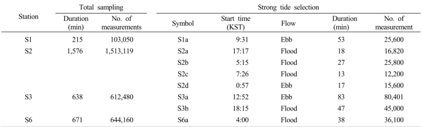
Fig 5 shows the resultant mean tidal velocity for 1 min

= 60 s resultant velocity (Fig. 4(B)) estimated from the 3-D data of east, north and depth velocity sampled at 16 Hz at Stations S2 and 6. Over the measurement period, the mean resultant velocity changed with tidal range while the flood velocity was greater than the ebb velocity.

The variation in velocity was represented as a kinetic en- ergy as the absolute mean value >1 min using the resultant velocity yielded by Eq. (2), and as a turbulence intensity as

the relative rate yielded by Eq. (3). The kinetic energy and turbulence intensity in relation to the mean resultant velocity at Station S3 are shown in Fig. 6. The kinetic energy E

or turbulence intensity (T

) can be expressed as a function of the resultant velocity by the following equations:

E

=E

(4)

T

=T

(5)

The turbulence intensity when the mean velocity was >0.2 m/s ranged between 10 and 50%, which was higher than the values of 8–15% recorded 4.7 m above the seabed at 22-m water depth in Puget Sound, USA and 10% recorded at a site off Seattle, USA (Thomson et al., 2012). The turbulence intensity affected the swimming speed of perch in tank ex- periments (Lupandin, 2005), and was the key variable affect- ing fish swimming in turbulent flow (Liao, 2007).

(A)

100 110 120 130

Elasped ime (s) -1.0

-0.5 0.0 0.5 1.0

Tidal velocity (m/s)

Vx Vy Vz

(B)

100 110 120 130

Elasped ime (s) -1.0

-0.5 0.0 0.5 1.0

Tidal velocity Vr (m/s)

200 250 300 350 400 450

Tidal direction A (deg)

Vr A

Fig. 4. 3-D tidal velocity, Vx east, Vy north, and Vz depth directions (A) and their resultant velocity and tidal direction (B) for the 16-Hz samples at S2b shown in Table 3.

(A)

15 20 25 30 35 40

KST (h) -1.0

-0.5 0.0 0.5 1.0

Tidal velocity (m/s)

65 70 75 80 85

Elevation D (m)

Vx Vy Um D

(B)

22 24 26 28 30 32

KST (h) -1.0

-0.5 0.0 0.5 1.0

Velocity (m/s)

67 68 69 70 71

Elevation D (m)

Vx Vy Um D

Fig. 5. Mean tidal flow indicated by easterly (Vx), northerly (Vy) and resultant velocity (Um) sampled at 16 Hz for 1 min at Station S2 on 6 April 2012 (A), and at Station S6 on 30 March 2014 (B).

The intercept and slope along with correlation coefficients for Eqs. (4) and (5), respectively, are given in Table 3. Ek increased with increasing resultant velocity, while T

de- creased with increasing resultant velocity. Furthermore, the relationship between the resultant velocity and the kinetic energy and the resultant velocity and the turbulence intensity was significant (high correlation coefficient), with the ex- ception of the turbulence intensity at S1, which exhibited a lower correlation coefficient. Thus, the main features of the velocity change in turbulence can be expressed accu- rately with the kinetic energy as absolute values in relation

to the mean velocity rather than the relative values of turbu- lence intensity.

The turbulence kinetic energy at S3 was similar to the

~0.03 m

/s

recorded in the eastern English Channel at 20

m above the seabed at 60-m water depth at a maximum flow

velocity of 1 m/s (Korotenko and Senchev, 2011). In one

study, the turbulence kinetic energy was adopted as the main

cue in the reaction of blue crab at the post-larval stage in

tank experiments (Saiz, 1994; Welch et al., 1999), while in

another study, the turbulence kinetic energy was not consid-

ered in the effects of turbulence on the movements of swim

(A)

0.2 0.4 0.6 0.8

Mean velocity (m/s) 0.00

0.01 0.02 0.03 0.04 0.05 0.06 0.07

Kinetic energy (m /s )

0 50 100 150 200 250 300

Turbulence intensity (%)

Tr Ke

22

(B)

0 0.1 0.2 0.3 0.4 0.5 0.6 0.7 Mean velocity (m/s)

0.000 0.001 0.002 0.003 0.004 0.005 0.006

Kinetic energy (m /s )

0 10 20 30 40 50 60

Turbulence intensity (%)

Tr Ke

22

Fig. 6. Relationships between resultant mean velocity and turbulent kinetic energy (Ek) and turbulence intensity (Tr) at Stations S2 (A) and S3 (B).

ming salmon (Enders et al., 2003).

The FFT periodicity spectrum of the resultant velocity and flow direction for all sampling data from S2b are given in Fig. 7. Among the several peaks of period of <30 s, one domi- nant peak is observed around 10 s as a shorter period caused by oscillation of fishing gear or movements of fish. The short- er periods of velocity and direction produced by FFT ranged between 4 and 15 s, as shown in Table 4. Complex changes in tidal flow velocity with variations in flow direction have been observed to generally occur in near-bottom tidal flow (Roget et al., 2010; Walter et al., 2011). Because a shorter flow period could have greater effects on fish swimming or escape behavior (Kim et al., 2008), in this study we considered shorter only periods of ~10 s.

Table 3. The constants and slopes of the relationship between velocity (Vr) and kinetic energy (Ek) from Eq. (4) and Vr and the turbulence intensity (Tr) from Eq. (5)

Site Ek Tr n*

Eo a r To b r

S1 S2 S3 S6

0.0016 0.0141 0.0041 0.0053

1.62 0.77 1.06 1.19

0.80 0.45 0.76 0.65

7.47 11.9 6.42 7.68

-0.190 -0.615 -0.472 -0.372

0.29 0.62 0.72 0.46

215 1578 638 671 r: Correlation coefficient

*: Equal to sampling duration (min) in Table 2

Fig. 7. Periodicity of resultant velocity Vr (A) and tidal direction (B) given by FFT of data recorded at 16 Hz at Station S2b on April 6 2012.

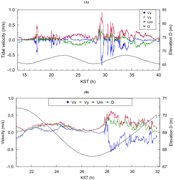
Fig. 8 shows the estimated period of velocity and direction

using the global wavelet spectrum (GWL) method (Torrence

and Compo, 1998) for the eight scenarios of strong tide for periods <30 s given in Table 2. The dominant period of veloc- ity and direction ranged between 4 and 17 s, while no peak period was present at S3a, S3b and S6a, as shown in Table 4.

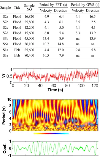
The complex periodicity of tidal flow was examined using the continuous wavelet method with Morlet in MATLAB as shown in Fig. 9. The period plumes are clearly visible for shorter periods of 3–6 s, represented in blue, and the curves of the correlation coefficients are shown in the plots at the bottom of the figure. Although, we were unable to plot the entire analyzed period for each scenario, the shorter period of each flow velocity or direction appeared between 3 and 20 s, similar to the results yielded by the global wavelet meth- od shown in Table 4. The periods produced by Morlet wavelet method for data recorded in Jiaozhou Bay, Qingdao, China at a water depth of 7 m and flow velocity of ~0.5 m/s with sampling at 16 Hz were estimated to be 4–64 s (Yuan et al., 2009). However, the periods produced by event detection method in the Eprapah Creek Estuary in eastern Australia at the seabed at a water depth of 2 m and flow velocity of

~0.25m/s with sampling at 50 Hz were estimated to be 0.25–1 s (Yuan et al., 2009). The results from these two studies are in agreement with the shorter periods of turbulent flow ob- served in our work. However, at a lower sampling rate of 2 Hz, the period at slack tide in Lunenburg Bay, Nova Scotia, Canada at a water depth of ~6 m and flow velocity of ~0.5 m/s ranged between 100 and 300 s (Rennie and Hay, 2008).

This longer period was also observed in our study using the global wavelet and FFT methods.

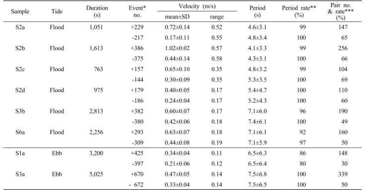
Tables 5 and 6 show the mean period, and the amplitude of velocity and direction, respectively, produced by peak event analysis for the eight scenarios of strong tide in Table 2. The mean periods ranged between 4 and 8 s for velocity and direction with no significant difference between flood and ebb tides. The amplitude of the velocity variation ranged be- tween 0.1 and 0.6 m/s and increased with increasing mean velocity. Similarly, the amplitude of the directional variation ranged between 20 and 90° and increased with increasing mean velocity. The period rate for peak or valley events ranged from at least 80 to 100% as covered time ratio of periodic events, while the pair rate of a consecutive pair of peak and valley events of period <30 s ranged between 30 and 70%. These rates are characteristic of the periodic ratios

in highly variable data of turbulence flow similar to the co- efficients yielded by the Morlet wavelet method. However, the peak event method can provide an estimate of the absolute range of amplitude for each period for comparison with other period analysis methods such as FFT or the wavelet method.

The amplitude obtained by peak event analysis was consid- ered as different terms in relation to the standard deviation, which was calculated for all data without periodic analysis (Bendat and Piersol, 2000).

(A)

0 5 10 15 20 25 30

Vr period (s) 0

0.1 0.2 0.3 0.4 0.5

Global wavelet spectrum

S1a S2a S2b S2c

S2d S3a S3b S6a

(B)

0 5 10 15 20 25 30

Direction period (s) 0

2000 4000 6000 8000 10000

Global wavelet spectrum

S1a S2a S2b S2c

S2d S3a S3b S6a

Fig. 8. Period of resultant velocity (A) and tidal direction (B) for eight scenarios of strong tide given in Table 2 estimated using global wavelet spectrum method.

Table 4. Peak period of tidal velocity and direction by FFT and the GWL method

Sample Tide SampleNO

Period by FFT (s) Period by GWS (s) Velocity Direction Velocity Direction S2a

S2b S2c S2d S3b S6a

Flood Flood Flood Flood Flood Flood

16,820 25,800 12,200 15,600 45,000 36,100

4.9 4.3 4.1 6.0 13.4 10.7

6.4 6.1 5.0 5.4 8.9 14.8

4.1 3.5 4.1 8.3 na na

16.5 2.5 4.1 13.9 13.9 na S1a

S3a Ebb Ebb

25,600 80,400

4.4 10.5

12.0 7.9

9.8 na

5.8 na

Fig. 9. Periodicities produced by continuous wavelet method with Morlet in MATLAB for resultant velocity Vr for 2000 sampling data (= 125s) at Station S2b. Colors from left to right represents higher periodic correlation, as shown in the plots at the middle of the figure.

The period frequencies of tidal velocity and tidal direction given by peak event analysis are shown in Fig. 10. When the minimum period was <1 s the peak periods ranged be- tween 2 and 4 s for the tidal velocity, and between 1 and 3 s for the tidal direction.

The period of the swim speed variation of fish depends on body length and tail beat frequency and has been variously reported at between 0.1 and several seconds (Videler and Wardle, 1991). The dominant period of swimming accel- eration in juvenile roundfish near the upper panel of the co- dend was 2~3 s at a towing speed of 1.5 m/s (Kim et al., 2008). The effect of turbulence on Atlantic salmon was inves- tigated at a dominant flow period of 6 s in tank experiments.

The dominant period of turbulence flow on the codend of the shrimp beam trawl or bottom trawl was estimated at be- tween 3 and 8 s when a shorter period of <60 s was selected (Kim, 2012; 2013a) and its value is possibly related to the period of swimming response in escaped fish from the codend (Kim et al., 2008). Therefore, period analysis of shorter peri- ods of a few seconds is suitable for studying the movements of swimming fish or fishing gear dynamics.

The turbulent water flow inside the codend could be re- sultant turbulence mixed up by tidal flow, towing motion of a fishing boat, wake of fishing gear, etc. In addition, the main index of turbulence effects on animal movements or swimming fish movements should be considered as kinetic energy, and the dominant period of tidal flow as 3-D and flow direction for analyzing the stability control of fish (Kim and Gordon, 2010; Webb and Cotel, 2010: Tritico and Cotel, 2010).

Therefore, in future, turbulent mixing inside the codend should be analyzed and interpreted as complex flow including the tidal turbulence flow in the overlying water.

(A)

0 2 4 6 8 10 12 14 16 18 20 22 24 Vr period by PEA (s)

0 5 10 15 20 25 30

Frequency (%)

S1a S2a S2b

S2c S2d S3a

S3b S6a

(B)

0 2 4

6 8 10 12

14 16 18 20

22 24 Direction period by PEA (s)

0 5 10 15 20

Frequency (%)

S1a S2a S2b

S2c S2d S3a

S3b S6a

Fig. 10. Period frequencies of tidal velocity (A) and tidal direction (B) produced by peak event analysis.

Table 5. Velocity period and amplitude produced by peak event analysis

Sample Tide Duration

(s) Event*

no.

Velocity (m/s) Period

(s) Period rate**

(%)

Pair no.

& rate***

mean±SD range (%)

S2a Flood 1,051 +229 0.72±0.14 0.52 4.6±3.1 99 147

-217 0.17±0.11 0.55 4.8±3.4 100 65

S2b Flood 1,613 +386 1.02±0.02 0.57 4.1±3.3 99 256

-375 0.44±0.14 0.58 4.3±3.1 100 66

S2c Flood 763 +157 0.65±0.10 0.35 4.8±3.2 99 104

-144 0.30±0.09 0.35 5.3±3.5 100 69

S2d Flood 975 +179 0.40±0.05 0.17 5.4±4.7 100 110

-186 0.24±0.04 0.17 5.2±4.3 100 60

S3b Flood 2,813 +382 0.60±0.07 0.17 7.1±6.0 96 190

　　　　　 -380 0.42±0.06 0.18 7.4±6.1 100 49

S6a Flood 2,256 +293 0.63±0.07 0.18 7.1±6.1 92 160

-309 0.44±0.08 0.19 7.1±5.9 97 50

S1a Ebb 3,200 +425 0.34±0.04 0.11 6.5±6.3 86 148

-397 0.21±0.06 0.12 6.5±6.4 80 30

S3a Ebb 5,025 +670 0.47±0.05 0.14 7.5±6.8 100 339

- 672 0.33±0.04 0.14 7.5±6.5 100 50

* + : Peak, -: valley

** Mean period × event no. / duration

*** Mean period × pair no. / duration

Table 6. Tidal direction period and amplitude produced by peak event analysis

Sample Tide Duration

(s) Event*

no.

Direction (°) Period

(s) Period rate**

(%)

Pair no.

& rate***

mean±SD range (%)

S2a Flood 1,051 +84 334±18 84 5.0±4.3 40 54

-175 61±102 87 5.8±4.8 97 27

S2b Flood 1,613 +315 315±13 59 4.4±3.5 85 218

-312 238±84 77 5.1±4.2 99 64

S2c Flood 763 +155 316±14 54 4.6±3.3 94 96

-139 256±65 59 5.5±4.7 100 64

S2d Flood 975 +167 297±6 33 5.8±4.5 100 104

-162 262±33 35 6.0±4.1 99 63

S3b Flood 2,813 +426 295±7 17 6.6±4.9 100 254

-437 277±16 18 6.3±4.8 98 58

S6a Flood 2,256 +360 315±12 18 6.0±5.1 95 198

-351 293±24 22 6.2±5.1 97 54

S1a Ebb 3,200 +366 80±19 18 7.4±6.1 84 176

-410 59±21 21 7.0±6.0 89 39

S3a Ebb 5,025 +857 77±6 19 5.8±4.5 99 483

-808 57±7 20 6.2±4.8 100 58

*, **, *** Refer to Table 5

Acknowledgement

Authors thank captain K.M. Bae and crews of the Research ship Charmbada, and Skipper H.D. Moon of the fishing boat for assistance of field measurements and Prof. B.K. Choi and Dr. D.S. Gu for useful help in periodicity analysis. Wavelet software for global wavelet spectrum was available at : http://paos.colorado.edu/research/wavelet/ provided by C.

Torrence and G. Compo. This work was supported by the Korea Research Foundation Grant funded by the Korean Government (NRF-2010-0022707).

References

Bendat JS and Piersol AG. 2000. Random data analysis and measure- ment procedures. 3^rdEdition.John Wiley & Sons, Inc. Hoboken, New Jersey. p.349-456.

Bernard PS and Wallace JM. 2002. Turbulent flow. Analysis, meas- urement and prediction. John Wiley & Sons, Inc. Hoboken, New Jersey. 497p.

Bouhoubeiny E, Germain G and Druault P. 2011. Time-resolved PIV investigations of the flow field around cod-end net structures. Fish Res 108, 344-355.(doi:10.1016/j.fishres.

2011.01.010)

Chanson H. 2010. Unsteady turbulence in tidal bores: Effects of bed roughness. J Waterway, Coastal & Ocean Eng 136, 247-256.

Chanson H, Reungoat D, Simon B and Lubin P. 2011. High-fre- quency turbulence and suspended sediment concentration measurements in the Garonne River tidal bore. Estua Coast

& Shelf Sci 95, 298-306.

Enders EC, Boisclair D and Roy AG. 2003. The effect of turbulence on the cost of swimming for juvenile Atlantic salmon (Salmo sala). Can J Aquat Sci 60, 1149-1160.(doi:10.1139/F03-101) Ham R van der R, Fontijn HL, Kranenburg C and Winterwerp JC.

2001. Turbulent exchange of fine sediments in a tidal channel in the Ems/Dollard estuary. Part I : Turbulence measurements.

Continen Shelf Res 21, 1605-1628.

Kim YH. 2012. Analysis of turbulence and tilt by in-situ measure- ments inside the codend of a shrimp beam trawl. Ocean Eng 53, 6-15. (http://dx.doi.org/10.1016/j.oceaneng.2012.06.014) Kim YH. 2013a. Analysis of the turbulent flow and tilt by in the

codend of a bottom trawl during fishing operation. Ocean Eng 64, 100-108. (http://dx.doi.org/10.1016/j.oceaneng.2013.02.019) Kim YH. 2013b. Shaking motion characteristics of a cod-end caused

by an attached circular canvas during tank experiments and sea trials. Fish Aquat Sci 16, 211-220.(http://dx.doi.org/

10.5657/FAS.2013.0211)

Kim YH and Gordon MS. 2010. Swimming and posture control of

common carp when penetrating mesh nets in water tunnel. Fish Res 102, 166-172.

Kim YH, Wardle CS and An YS. 2008. Herding and escaping re- sponses of juvenile roundfish to square mesh window in a trawl cod end. Fish Sci 74, 1-7. (http://dx.doi.org/10.1111/j.1444- 2906.2007.01490.x.)

Korotenko KA and Senchev AV. 2011. Turbulence investigation in a tidal coastal region. Oceanography 51, 394-406.

Liao JC. 2007. A review of fish swimming mechanics and behaviour in altered flows. Phil Trans R B 362, 1973-1993. (http://dx.do- i.org/10.1098/rstb.2007.2082)

Liu H, Wu C and Wu J. 2009a. Contrast between estuarine and river systems in near-bed turbulent flows in the Zhujiang (Pearl River) Estuary, China. Estuar. Coast Shelf Sci 83, 591-601.

Liu Z, Wei H, Lozovatsky ID and Fernando HJS. 2009b. Late summ- er stratification, internal waves, and turbulence in the Yellow Sea. J Mar Syst 77, 459-472.

Lozovastsky I, Liu Z, Fernando H, Armengol J and Roget E. 2012.

Shallow water tidal currents in close proximity to the seafloor and boundary-induced turbulence. Ocean Dyna 62, 177-191.

(DOI:10.1007/s10236-011-0495-3)

Lupandin AI. 2005. Effect of flow turbulence on swimming speed of fish. Biol Bull 32, 461-466.

McLelland SJ and Nicholas AP. 2000. A new method for evaluating errors in high-frequency ADV measurements. Hydrol Proce 14, 351-365.

Narasimha R, Kumar SR, Prabhu A and Kailas SV. 2007. Turbulent flux events in a nearly neutral atmospheric boundary layer.

Philos Trans R Soc A 365, 841-858. (http://dx.doi.org/

10.1098/rsta.2006.1949)

O’Neill FG, McKay S, Ward JN, Strickland A, Kynoch RJ and Zuur AF. 2003. An investigation of the relationship between sea state induced vessel motion and cod-end selection. Fish Res 60, 107-130. (http://dx.doi.org/10.1016/S0165-7836(02)00056-5) Parra SM, Marino-Tapia I, Enriquez C and Valle-Levinson A. 2014.

Variations in turbulent kinetic energy at a point source sub- marine groundwater discharge in a reef lagoon. Ocean Dyna (doi:10.1007/s10236-014-0765-y)

Pichot G, Germain G and Priour D. 2009. On the experimental study of the flow around a fishing net. J Mech B/Fluids 28, 103-116.

(http://dx.doi.org/10.1016/j.euromechflu.2008.02.002)

Rennie CD and Hay A. 2008. Reynolds stress estimates in a tidal channel from phase-wrapped ADV data. J Coastal Res 26, 157-166.

Rippeth TP, Simpson JH, Williams E and Inall ME. 2003.

Measurements of the rates of production and dissipation of tur- bulent kinetic energy in an energetic tidal flow: Red Warf Bay revisited. J Phys Oceanogr 33, 1889-1901.

Roget E, Planella J, Fernando HJS and Liu Z. 2010. Intermittency

of near-bottom turbulence in tidal flow on a shallow shelf.

Geophysical Res Oceans 115, C05006. 16p.

Saiz E. 1994. Observations of the free-swimming behaviour of Acartia tonsa: Effects of food concentration and turbulent wa- ter motion. Limnol Ocean 39, 1566-1578.

Seena A and Sung HJ. 2011. Wavelet spatial scaling for educing dynamic structures in turbulent open cavity flows. J Fluids Struct 27, 962-975.

Shadwick RE and Lauder GV. 2006. Fish biomehcnics. Fish physiol- ogy vol. 23. Academic Press. San Diego, USA. 542p.

Simpson JH, Williams E, Brasseur LH and Brubaker JM. 2005. The impact of tidal straining on the cycle of turbulence in a partially stratified estuary. Continen Shelf Res 25, 51-64.(doi:10.1016/

j.csr.2004.08.003)

Thomson J, Polagye B, Durgesh V and Richmond MC. 2012.

Measurements of turbulence at two tidal energy sites in Puget Sound, WA. IEEE J Oceanic Eng 37, 363-374.(DOI:10.1109/

JOE.2012.2191656)

Thorpe SA. 2007. An introduction to ocean turbulence. Cambridge Univ. Press. UK. Ch. 1.(1-36) Ch.2(37-76) P. 267.

Thorpe SA, Green JAM and Simpson JH. 2008. Boils and turbulence in a weakly stratified shallow tidal sea. Am Meteorol Soc 38, 1711-1730.(DOI:10.1175/2008JPO3931.1)

Torrence C and Compo GP. 1998. A practical guide to wavelet analysis. Bull Am Meteorol Soc 79, 61-78.(http://dx.doi.org/

10.1175/1520-0477(1998)079<0061:APGTWA>2.0.CO;2) Tritico HM and Cotel AJ. 2010. The effects of turbulent eddies on

the stability and critical swimming speed of creek chub

(Semotilus atromaculatus). J Exp Biol 213, 2284-2293.(doi:

10.1242/jeb.041806)

Videler JJ and Wardle CS. 1991. Fish swimming stride by stride:

speed limits and endurance. Rev Fish Biol & Fish 1, 23-40.

Walter RK, Nidzieko NJ and Monismith SG. 2011. Similarity scaling of turbulence spectra and cospectra in a shallow tidal flow.

J Geophysical Res Ocean 116, C10019. 14p.

Webb PW and Cotel AJ. 2010. Turbulence: Does vorticity affect the structure and shape of body and fin propulsors? Integ Comp Biol 50, 1155-1166.(http://dx.doi.org/10.1093/icb/

icq020)

Welch JM, Forward jr RB and Howd PA. 1999. Behavioral responses of blue crab Callinectes sapidus postlarvae to turbulence:

Implications for selective tidal stream transport. Mar Ecol Prog Ser 179, 135-143.

Yuan Y, Wei H, Zhao L and Cao Y. 2009. Implications of inter- mittent turbulent bursts for sediment resuspension in a coastal bottom boundary layer: A filed study in the western Yellow Sea, China. Mar Geol 263, 87-96.(doi:10.1016/j.margeo.

2009.03.023)

Zhang Q, Xu CY and Chen YD. 2010. Wavelet-based character- ization of water level behaviors in the Pearl river estuary, China Stoch Environ Res Risk Assess 24, 81-92.

2014.10.29 Received

2014.11.20 Revised

2014.11.21. Accepted