A Cluster Analysis for Housing Submarkets Considering Spatial Autocorrelation

(1)

1. Introduction

1.1 Background and purpose

Locational fixednessof housing creates a unique spatial characteristic in the region where it is located, thus housing market of an urban area necessarily shows attributes which aredivided regionally. That is, a housing market in an urban area is a combination of regionally different submarkets and not just a single market. Because there are various submarkets, a housing policy should reflect the attributes of each submarket. However, housing policy of Korea has been enforced in a national level of gross housing market or dual separation, which is metropolitan area and non‐metropolitan area. Regionally different responds accompany negative evaluation to government’s housing policy. Therefore, to makea more effective housing policy, a new approach to regionally different housing submarket is needed.

According to this need, researches for housing submarkets have beenconsistently proceeded. Kim and Park(2003) showed there was a distinct

difference when housing submarkets are classified by housing trade and price change rate, and demonstrated separate housing submarkets by analyzing housing price change rate targeting Seoul and neighboring apartment. Kim and Woo(2004) separated housing market as several submarkets, estimated hedonic price function in each housing submarket and verified its usefulness. Kang(2008) classified and analyzed housing submarkets, and suggested housing policies considering characteristics of each class. Hong(2009) performed factor analysis, one‐way ANOVA, cluster analysis, and separated metropolitan housing market into 6 submarkets. Song and Jang(2010) performed cluster analysis according to regional attributes, separated housing market types of Seoul Metropolitan area, and tried to understand characteristics according to these types.

However, the biggest problem of these researches is that they do not consider spatial autocorrelation of the housing location. Spatial autocorrelation means that the value distribution of a specific area within a study area affects neighbor areas of that specific area

Received: 2016.05.31, revised: 2016.06.28, accepted: 2016.06.30

* MemberㆍPh. D. Student, Department of civil and Environmental Engineering, Seoul National University, [email protected]

** MemberㆍProfessor, Department of civil and Environmental Engineering, Seoul National University, [email protected]

*** Corresponding authorㆍResearch Professor, Department of civil and Environmental Engineering, Seoul National University, [email protected]

A Cluster Analysis for Housing Submarkets Considering Spatial Autocorrelation

1)

Lee, Bae Sung*ㆍYu, Ki Yun**ㆍKim, Ji Young***

Abstract

A housing market in an urban area is not just a single market but a combination of regionally different submarkets.

This study begins with a critical mind that previous researches did not consider the spatial autocorrelation of each area where the housings are located. The clustering analysis of housing submarket which considers spatial autocorrelation is performed as it follows. First, 4 housing market attribute variables are reducted to 1 variable by principle component analysis. Then, after calculating Gi

^*

max by AMOEBA, 7 housing submarkets which have similar characteristics based on Gi

^*

max are classified. The characteristics of each submarket are investigated, then political implication is deduced as the following. Different level of housing policy should be made to each cluster because each cluster has different level of spatial autocorrelation.

Keywords : Housing Submarket, Cluster Analysis, Principle Component Analysis, Spatial Autocorrelation

63 Vol.24 No.2 June 2016 pp.63-70

Research Paper

ISSN: 2287-6693(Online) http://dx.doi.org/10.7319/kogsis.2016.24.2.063

(2)

to have similar value distributions. Without considering spatial autocorrelation, spatial dependence and spatial interaction within many socioeconomic phenomena are totally ignored.

The difference of this study is that it performs cluster analysis using a new methodology which supplements previous method. That is, this study investigates a possibility of a new cluster analysis considering spatial autocorrelation for statistical classification of housing submarkets.

Therefore, the purpose of this study is to suggest a cluster analysis for housing submarkets considering spatial autocorrelation and finding a political implication. Also another purpose is making a base data for regionally different level of housing policy, by showing there exist different autocorrelation levels of clusters,

1.2 Scope and method of research

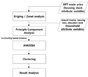
Before selecting data of this study, previous reviews are referenced and characteristics of regional housing markets are regarded as a combinationof characteristics of housing stocks and social economic characteristics of household. Then, housing price, annual household income, household housing loan, household head educational level are chosen as variables. Spatial scope of research is aimed at 423 admi nis trati ve don g of Seoul. AM OEBA( A Multidirectional Optimal Ecotope‐Based Algorithm)

Figure 1. Flow of this study

method is adapted to consider spatial dependence by spatial autocorrelation. To apply this method, the characteristic of housing market has to be a single variable. Therefore, variables selected above are reducted to a single variable by principle component analysis. Then, that variable is inserted into AMOEBA method, and clustering is performed by the Gi

^*

max which is the output of AMOEBA. Fig. 1 is the sequence of this study.

2. A clustering analysis considering spatial autocorrelation

In this research, Gi

^*

max which is calculated by AMOEBA procedure is used for a cluster analysis.

Since these Gi

^*

max values get to bediscretely distributed in groups, proper numbers of intervals are decided by considering the discreteness in the whole data. After group‐matching of Gi

^*

max values in each interval, a cluster analysis can be accomplished by the degrees of classified spatial autocorrelation.

Before calculating Gi

^*

max, the principle of AMOEBA should be looked into. This method is performed by Gi

^*

(Getis and Ord, 1992), which is one of LISA(Local Indicators of Spatial Association).

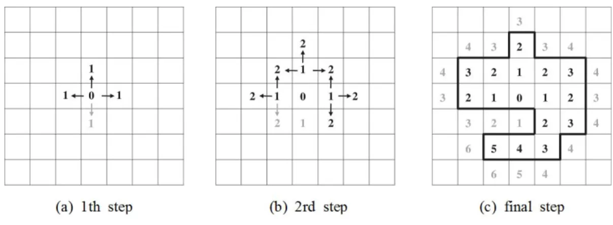
First, Gi

^*

is calculated in the start cell, and the

statistic is put as a Gi

^*

(0). Gi

^*

is also calculated in

the start cell and neighbor cells, then the statistics are

put as a Gi

^*

(1). If Gi

^*

(0) is bigger than 0 and the

biggest value between these Gi

^*

(1) is bigger than

Gi

^*

(0), the area which shows the biggest value is

designated as a primary cluster. Fig. 1(a) shows the

area added in the center cell with 3 other cells which

are upper, left, right cells. These cells arechosen as

a 1st step cluster. These processes are repeated until

there is no more increase of Gi

^*

by adding new cell

(if Gi

^*

(0) is bigger than 0). After going through 4~6

steps, the final cluster is deduced like Fig. 1(c). The

bold line including these areas shows a final shape of

the cluster(Lee et al., 2010). Also, in case Gi

^*

(0) is

smaller than 0, when the same process is applied, 3

kinds of area (the cluster of high values and the

cluster of low values, and outside of cluster) are

deducted.

(3)

Figure 3. the result of AMOEBA (Aldstadt and Getis, 2006)

So far, AMOEBA method is mainly used to delimitate proper spatial cluster with retaining spatial agglutinability(Lee et al., 2011; Kwon et al., 2015).

However, by using Gi

^*

max, the calculation result of AMOEBA, a cluster analysis for the whole research area can be implemented.

In the process of each cell drawing cluster boundary of maximum Gi

^*

, each cluster has no choice but to be overlapped. By putting the maximum Gi

^*

to Gi

^*

max, and mapping, Gi

^*

max draws the picture of spatial autocorrelation by adding up all the Gi

^*

(Jankowska et al, 2008). This means that the spatial autocorrelation map shows positive and negative intensity according to Gi

^*

max. This method makes possible the drawing of clusters for all cells in a proper way like Fig. 4. Finally, by proper categorization, Gi

^*

max from AMOEBA can be used

Figure 4. Cluster analysis considering spatial autocorrelation (Jankowska et al., 2008)

for cluster analysis considering spatial autocorrelation of univariate data.

3. Experiment and application

3.1 Experiment data

An experiment is designed as it follows. For classifying housing submarkets targeting 423 administrative‐dong of Seoul, cluster analysis considering spatial autocorrelation is applied. That is, for investigation possibility of housing submarket analysis in the microscopic spatial unit, which is the administrative dong level, data is composed by considering the obtainability and build‐up possibility.

Meanwhile, previous study shows that housing

submarkets are defined by adding characteristics of

Figure 2. AMOEBA procedure (Lee et al., 2010)

(4)

housing stock and socialeconomic ones of household(Park et al., 2012). Referencing this, to obtain different housing political implication per cluster, data isgathered by dividing two sides which are housing stock attributes in the supply side and household socio‐economic attributes in the demand side. That is, housing trade price is chosen by consideringthe abounding obtainability ofactual data and applicability of kriging in housing stock attribute.

And variables such asannual household income, housing loan, population ratio per education level, are chosen with priority given to household economic condition which has the biggest effect on housing demand. After the standardization of average value of these 4 variables per administrative‐dong, data is inserted in the administrative‐dong layer of Seoul as an attribute for experiment.

For housing trade price variable, raw datais classified as 3 categories which are small size(under 60 m

²

), medium size(over 60 m

²

~ under 85 m

²

), and large size (over 85 m

²

~ under 135 m

²

). Medium size is assumed to represent all housing size, because by using small size, price per area can be calculated excessively. Also, by using large size, price per area can be underestimated. Data from the period between November 2014 and October 2015 is selected and converted into 10 thousand won / m2. Each data for household social · economic characteristic variables is

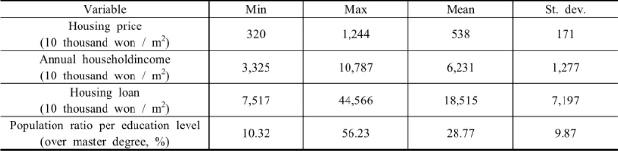
downloaded from ‘K‐atlas’, the GIS based real estate solution developed by ‘Real estate 114’ and converted. Basic statistics for each variable are shown in Table 1.

3.2 Principle component analysis

For the AMOEBA procedure, variables are converted to Z‐score, and a single principle is extracted by principle component analysis. To verify principle component analysis, Kaiser‐Meyer‐Oklin (KMO) test and Bartlett test are executed. The results are as follows. KMO value is 0.799, which shows selection of variables is good. P‐value of Bartlett test is 0.000, which is smaller than significance level of 0.05. This shows there exists common factor between variables. Correlation coefficient matrix between variables is shown in Table 2. P‐values of each component are 0.000 which is smaller than thesignificance

Table 3. Extracted principle component and its loading

Variable Loading

Housing price .894

Annual household income .859

Housing loan .933

Population ratio per education

level .872

Eigen value 3.169

Explanation quantity to total

variance(%) 79.231

Variable Min Max Mean St. dev.

Housing price

(10 thousand won / m

²

) 320 1,244 538 171

Annual householdincome

(10 thousand won / m

²

) 3,325 10,787 6,231 1,277

Housing loan

(10 thousand won / m

²

) 7,517 44,566 18,515 7,197

Population ratio per education level

(over master degree, %) 10.32 56.23 28.77 9.87

Table 1. Basic statistics of variables

Variable Housing price Annual household

income Housing loan Population ratio per edu‐level

Housing price 1 .633 .832 .709

Annual household income .633 1 .755 .679

Housing loan .832 .755 1 .723

Population ratio per edu‐level .709 .679 .723 1

Table 2. Correlation coefficient matrix

(5)

level of 0.05. Correlations between each variable are strong, which show variables are suitable for principle component analysis. Extracted principle component and its loading are shown in Table 3.

3.3 Housing submarkets cluster analysis There is no consensus for what number of classification is optimal, and which variable is suitable for submarket separation(Kim, 2004).

Therefore, this study classifies housing submarket of Seoul as 7 categories based on experimental result.

This means that Gi

^*

maxvalues are divided into 7 intervals in groups discretely(Fig. 4, Table 4). The reason why submarkets are determined to 7 intervals is as follows. Gi

^*

max was scattered discretely and there were 7 groups whereGi

^*

maxes were gathered sparselyfrom the scatter plot. In Cluster 1, Gi

^*

max is

‐8.370210 and north‐eastern area of Seoul is mostly

included into the cluster. In Cluster 2, the scope of Gi

^*

max is from ‐8.370209 to ‐7.106010 and south‐

western area of Seoul is mainly included. In Cluster 3, the scope of Gi

^*

max is from ‐7.106009 to ‐ 3.052499 and north‐western area is chiefly included.

In Cluster 4 and 5, the scope of Gi

^*

max is respectively from ‐3.052498 to 15.674370 and from 15.674371 to 15.933147. Cluster 4 and 5 show a very small size of clusters, which is composed by 1~

5 dongs, which are lied around and not agglomerated in a specific area. In Cluster 6, the scope of Gi

^*

max is from 15.933148 to 16.212199 and downtown area and its surroundings are included in the cluster. In Cluster 7, the scope of Gi

^*

max is 16.212200 and Gangnam 3 gu and few adjacent dongs are included to the cluster.

Figure 5. Result of cluster analysis for housing submarket

(6)

4. Result analysis

4.1 Characteristic analysis per housing submarkets

Investigation for each housing submarket by clustering is conducted. In cluster 1, Gi

^*

max is ‐ 8.370210 which is the biggest negativevalue between all Gi

^*

max values, so the regions in the cluster show very strong positive spatial autocorrelation. These are the areas where original variables (housing price, annual household income, housing loan) are gathered together and the low values are the most strongly surrounded by low values. In cluster 2, Gi

^*

max is from ‐8.370209 ~ ‐7.106010, the regions in cluster show relatively strong positive spatial autocorrelation.

These are the areas where original variables (housing price, annual household income, housing loan) are gathered together andwhere the low values are surrounded by low values relatively strongly. In cluster 3, the areas in cluster show relatively weak positive spatial autocorrelation. Since the assigned administrative‐dongs are gathered together in a specific area, the cluster detection was relatively easy. In cluster 4, 5, the areas in the cluster show weak positive spatial autocorrelation. Since the assigned administrative‐dongs are scattered sporadically in many areas of Seoul, the visual

cluster detection is relatively hard. The areas are characterized as a transitional zone because 4 variables do not show relatively distinguishing relationship. In cluster 6, the regions in cluster show relatively strong positive spatial autocorrelation.

These are the areas where original variables (housing price, annual household income, housing loan) are gathered together and the high values are surrounded by high values relatively strongly. In cluster 7, the regions in cluster show very strong positive spatial autocorrelation. These are the areas where original variables (housing price, annual household income, housing loan) are gathered together and the high values are very strongly surrounded by high values.

4.2 Political implication

Political implication considering the research result is as the following. Since the degrees of spatial autocorrelation differ from housing submarkets to submarkets, different level of housing policy should be made considering the degrees of spatial autocorrelation. In cluster 1, 7, since the areas in the cluster have a very strong positive spatial autocorrelation, the housing policy should consider interdependence and interaction between areas in those clusters. However, in cluster 4, 5, since the areas in cluster have a very weak positive spatial

Clusters Included areas

Gi^*

max

total Administrative‐dong

Cluster 1 95

Gangbuk‐gu bun‐dong, etc(12), Nowon‐gu wolge1‐dong, etc(12), Dobong‐gu ssangmoon1‐dong, etc(12), Sungbook‐gubomoon‐dong, etc(8), and so on

‐8.370210

Cluster 2 104 Gangsu‐gudungchon‐dong, etc(14), Yangchun‐gusinwol‐dong, etc(9), Gooro‐gugooro‐dong, etc(12), Gumchun‐gugasan‐dong, etc(10), and so on

‐8.370209 ~

‐7.106010 Cluster 3 43 Eunpyung‐guboolgwang‐dong, etc(15), Mapo‐guhapjung‐dong, etc(6),

Suhdaemoon‐gu, yeonhee‐dong(10), and so on

‐7.106009~

‐3.052499 Cluster 4 47 Gangdong‐gugildong, etc(9), Songpa‐gusamjun‐dong, etc(9),

and so on

‐3.052498~

15.674370 Cluster 5 37 Sungdong‐gusakun‐dong, etc(7), Gangdong‐gugangil‐dong, etc(8), and so

on

15.674371~

15.933147 Cluster 6 11 Jongro‐gusajik‐dong, etc(5), Joong‐gusogong‐dong, etc(3),

and so on

15.933148~

16.212199

Cluster 7 84

Gangnam‐gusinsa‐dong, etc(19), Seocho‐gujamwon‐dong, etc(16), Songpa‐guoryun‐dong, etc(14), Yungdunpo‐gumoonrae‐dong, etc(4), Mapo‐guahyun‐dong, etc(6), and so on

16.212200

Table 4. Included areas per cluster and Gi

^*

max

(7)

autocorrelation, housing policy does not need to consider interdependence and interaction between the areas in those clusters.

Meanwhile, Seoul local government has provided public rental house in earnest since late 1980s.

Nowadays, Seoul local government is trying to provide public rental house in many ways. When considering the moving‐in qualification to public rental house, different levels of housing policy should be applied according to the strength of spatial autocorrelation in terms of ‘Social Mix’. For example, in cluster 1, 7, the people who have stayed in these areas can get incentives when moving to other cluster for the mixing of social stratum.

However, the areas in cluster 4, 5 can be regarded as desirable in terms of social mix. Contrary to cluster 1, 7, the people who have stayed in cluster 4, 5 should get incentives, when moving to same cluster in terms of social mix. In the same view, for cluster 2, 3, 6, by applying different level of housing policyfor public rental house to each cluster according to the strength of spatial autocorrelation, the people who move in the public housing can be broken up into a waywhich weakens spatial autocorrelation within the cluster, and‘Social Mix’ of Seoul can be achieved eventually.

5. Conclusion

This study shows a series of analysis in the objective of classification of housing submarkets considering spatial autocorrelation. For cluster analysis, targeting 423 administrative‐dong of Seoul, 4 characteristic variables of housing market arereducted to a single variable by principle component analysis. After processing AMOEBA method, 7 housing submarkets are classified according to Gi

^*

max. Characteristics per housing submarkets are investigated and political implication that different level of housing policy per cluster should be established is deduced.

Meanwhile, the limitations of this study are the followings. To use AMOEBA, the data should be as small as administrative‐dong level. However, only 4 variables were inserted to AMOEBA because these

were the only administrative‐dong level data in Korean public/private research institutes. Because of the acquisition limitation of these explanatory variables, making more accurate cluster was hard.

For example, due to the lack of explanatory variables, moonrae‐dong, ahyun‐dong are included with Gangnam in cluster 7. In the subsequentresearch, adding more explanatory variables, or other clustering method considering spatial autocorrelation are needed.

Also, this study does notanalyze the proper number of cluster for accurate classification, and a criterion for judging cluster number indirectly per individual spatial data is needed.

Acknowledgement

This research was supported by a grant (15CHUD‐

C061156‐05) from the National Spatial Information Research Program funded by the Ministry of Land, Infrastructure and Transport of the Korean government.

References

1. Kang, P. M., 2008, A study on the characteristics of housing sub-markets in Seoul: focusing on housing tenure and housing types, Doctoral thesis, Kyongwon University.

2. Kim, G. S. and Park, J. Y., 2003, The spatial pattern of housing prices; Seoul and new towns, Journal of the Korean Regional Science Association, Vol. 9, No. 1, pp. 47-61.

3. Kim, J. Y. and Woo, K., 2004, Housing submarket analysis of the capital region, The Korea Spatial Planning Review, Korea Research Institute for Human Settlements, Vol. 41, pp. 101-111.

4. Kwon, P. and Yu, K., 2015, Trade area delimitation using AMOEBA technique, Journal of the Korean Society for Geospatial Information System, Vol. 23, No. 2, pp. 11-16.

5. Park, K. H., Ryu, Y. T., Jung, H. J. and Lee, Y, K., 2012, Urban social geography: an introduction, Sigma press.

6. Song, M. K. and Jang, H., 2010, Characterization of

cities in Seoul metropolitan area by cluster analysis,

(8)

Journal of the Korean Society for Geo-spatial Information System, Vol. 18, No. 1, pp. 45-52.

7. Lee, J. H., Kim, S. I., Han, K. S. and Lee, Y. W., 2011, Hotspot detection for land cover changes using spatial statistical methods, Korean Journal of Remote Sensing, The Korean Society of Remote Sensing, Vol. 27, No. 5, pp. 601-611.

8. Lee, S. I., Cho, D. H., Sohn, H. K. and Chae, M.

O., 2010, A GIS-based method for delineating spatial clusters: a modified AMOEBA technique, Journal of Korean Geographical Society, Korean Geographical Society, Vol. 45, No. 4, pp. 502-520.

9. Hong, S. M., 2009, A study on the characteristics of housing markets in the metropolitan area, Doctoral thesis, Kyongwon University.

10. Aldstadt, J. and Getis, A., 2006, Using AMOEBA to create a spatial weight matrix and identify spatial clusters, Geographical Analysis, Vol. 38, No. 4, pp.