Optimal Sizing of In-Plant and Leased Storage Spaces under a Randomized Storage Policy

임의 저장방식 하에서 기업 내 저장공간과 외부의 임차공간에 대한 최적 규모 결정

이 문 규^†

계명대학교 산업시스템공학과

Optimal Sizing of In-Plant and Leased Storage Spaces under a Randomized Storage Policy

Moon-Kyu Lee

Department of Industrial and Systems Engineering, Keimyung University, Daegu, 740-701

This paper considers a trade-off effect between in-house storage space and leased storage space in generic warehouses operated under a randomized storage assignment policy. The amount of in-house storage space is determined based on the law of large numbers satisfying a given service level of protection against space shortages. Excess space requirement is assumed to be met via leased storage space. A new analytic model is formulated for determining the excess space such that the total cost of storage space is minimized. Finally, computational results are provided for the systems where the standard economic-order-quantity inventory model is used for all items.

Keywords: warehouse leasing, storage capacity, randomized storage policy, optimization

†Corresponding author : Professor Moon-Kyu Lee, Department of Industrial and Systems Engineering, Keimyung University, Daegu, 740-701, Korea, Fax : +82-053-580-5165, E-mail : [email protected]

Received April 2004; revision received August 2004; accepted September 2004.

1. Introduction

A supply chain is referred to as an integrated network which synchronizes a series of interrelated business process including procurement, inventory, manufacturing, logistics, distribution, and sales. For the past decade, supply chain management has attracted a great deal of attention to business managers who try to seek effective tools to enhance the entire spectrum of their business process from suppliers to end customers by treating it as a whole process. Therefore, interactions among the participants in the supply chain are considered to be more important than those within each participant. The interactions among suppliers, manufacturers, and distributors are usually coordinated by preparing inventories of raw materials or final products.

Not long ago, most manufacturers have had their own private warehouses which store all inventories including law materials, work in process, and final products. The primary reasons are

convenience in material handling and transportation cost reductions. However, recently there has prevailed a trend that manufacturers focus on their core activities by outsourcing some of warehousing functions to third parties. Cost reduction in material handling and enhanced customer satisfaction by the prompt response from outside warehouses near the customers are some of the advantages expected for warehouse outsourcing.

Therefore, the two warehousing options, private warehousing and warehouse outsourcing, has to be reasonably compromised to secure such advantages.

The storage assignment policy is one of the major factors that influence the amount of storage space needed. The storage policy defines the way of assigning items to storage locations. There are three different storage policies used frequently in practice. They are randomized storage (RAN), class-based storage (CN), and full turnover-based storage (FULL).

Previous studies on the determination of storage capacity considering storage policies are very scarce. Early studies on this area include Rosenblatt and Roll (1984, 1988), Roll et al.

(1989), and Francis et al. (1992). Analytical and/or simulation models for determining the storage size under RAN were presented in their studies. Especially, Francis et

al. (1992)introduced mathematical models for determining

the storage capacities while either satisfying a desired service level or minimizing costs related to owned warehouse space and leased one.

On the contrary, seeking a compromise between private warehousing and contracting storage space has been substantially tried during the past few decades. As far as we know, the first study related to the warehouse sizing problem considering space leasing was done by White and Francis (1971). They formulated the sizing problem as a multi- variable discrete optimization problem which can be solved as a linear programming problem. Later, Lowe et al. (1979) extended the wok of White and Francis (1971) to additionally incorporate expansion and contraction costs. Cormier and Gunn (1996a) presented models for a static problem incorporating inventory policy cost, warehouse cost, and the cost associated with leasing space from outside sources. A similar study without consideration of warehouse leasing was made by the same authors (1996b). Jucker et al. (1982) investigated a static problem with stationary demand over a planning horizon to determine the capacities of a single production plant and a set of regional leased warehouses which maximize expected profit. A trial-and-error method was presented by Ballou (1999) to seek the best combination of private-public warehouse size alternatives. Hung and Fisk (1984), and Rao and Rao (1998) considered the same static problem. Cormier and Gunn (1992) give a review of existing storage capacity models.

Recent models for optimizing multi-period warehousing contracts under random space demand are presented by Chen

et al.(2001). Zhou et al.(2001) considered a problem of

allocating customer demand to primary and secondary warehouses with capacity restrictions. The role of the secondary warehouses is to back up the primary warehouse that is depleted with needed safety stocks. They formulated the problem as an integer programming model and suggested a genetic algorithm to solve the problem. Lee (1999, 2001) analytically investigated the effect of the storage policies on the storage capacity while allowing external storage space leasing and satisfying a desired service level. Algorithms presented in Lee (1999, 2001) determine the optimal storage capacity under the two storage policies, RAN and CN, such that the total cost of owned and leased storage space per unit time is minimized while satisfying a given service level. In

this paper, for RAN we present a new way of estimating the excess storage amount incurred by available storage-space shortages, which is different from those by Lee (1999, 2001)

2. Estimating Excess Storage Space

We consider two alternatives of warehousing, leased warehousing and private warehousing. Under leased warehousing, warehouse storage space is contracted on a storage volume per unit time basis and may require some investment for handling equipments if they are owned and operated by customers. Here, we assume the planning horizon is a single period. Since costs incurred by each alternative are different, we need to determine the most economical combination of the two warehousing alternatives. Note that public warehousing can be considered to be a special case of leasing where there are no fixed charges (Ballou, 1999).

With RAN, incoming items are equally likely to be stored in any storage location when a storage operation is carried out. In practice, an incoming storage load is often placed in the open location closest in time to the input/output pointof the warehouse to which incoming and outgoing loads are transferred. This storage rule is called

ꡒ

closest-open- location

ꡓ

rule. If some conditions like high utilization of the storage locations are met, the warehouse system behaves in the same manner as RAN dose (Hausman, 1976; Francis et

al., 1992). Hence, most of actual warehousing systems can

be modeled by assuming RAN.

One obvious advantage of RAN will be better utilization of storage space than other storage policies such as dedicated storage policiesunder which a storage location is assigned dedicatedly to a specific item. This advantage in turn leads to smaller storage space required than that under dedicated storage.

Since items can be stored in any available locations, the required storage capacity for RAN will be equal to the maximum of the aggregate inventory level for all items to be stored. However, in real situations, to exactly predict the aggregate inventory level is very difficult due to the dynamic nature of the replenishment process and retrieval operation of items.

In this paper, we assume that the inventory level of item i,

X

i, i=1, ..., n follows a uniform distribution, U(ai, bi). The economic order quantity (EOQ) model will be one example of the uniform distribution. If all items are replenished at the same time, the aggregate inventory level, X, of the overall system will be

_∑

ⁿ

i = 1

X

i. However, if we carefully schedule

the replenishment time of each item, then the aggregate inventory level can be considerably reduced, and so can the total storage requirement of the warehouse.

Now, let ti be the replenishment time of item i, then Page and Paul (1976) showed that the replenishment time and the minimum of the aggregate inventory level, Xlb, are given by

t

i

=

_{  }



^

^

^

^/

_{  }



^

^

^

, i = 1, ..., n,

X

lb

=

_{  }



^ _{  }



^

^

^

^

^

^/

_{  }



^

^

^

where items are numbered arbitrarily, and t1 = 0. However, this replenishment schedule may be too sophisticated and tight to follow in most real situations. Therefore, in this paper we consider the simple case where the first replenishment times of all the items are set to be at time zero, the starting point of time. In this case, the storage capacity will be the maximum which can be used as an upper bound for the first cut design of the warehouse. Then, by the central limit theorem, when the number of items is sufficiently large, the aggregate inventory level follows approximately a normal distribution.

Let A =

_{  }^{ }

^{, B =}

_{  }^{ }

, and Z = (X-



_{) /}



_where



= (A+B)/2 and



_{= (}

_{  }



^

^

^

^{ }

^

^

^

^{ }

^

^.

Then, since n is large, Z follows the standard normal distribution, N(0,1).

The service level of the in-house (i.e., private) warehousing system is given as 1-α (0<α<1), which α implies a probability of a space shortage occurring (hereafter, we call it the shortage probability). If the storage requirement is greater than the storage capacity, a space shortage occurs. Under such conditions, the excess space requirement is to be met via leased storage space. Therefore, the probability that X exceeds the storage capacity at the 1-α service level, S(α), is less than or equal to α.

Assuming the independent replenishment of the items, we first present a model for estimating the excess storage amount incurred by available-storage-space shortages. Based on that amount we can determine the economic storage capacity which is large enough to accommodate the incoming items with probability greater than or equal to (1- α0).

By the normal-distribution property of Z, the storage capacity can be represented by a function of the unknown variable, α:

S(

α

) =



₊

za

 

where α≦α0, and za is determined by Pr(Z>za) = α for 0≦

α≦1. Throughout this paper, we consider the case where α0

≦0.5, which may be valid for most warehouses in practice.

Lee (1999, 2001) computed the expected amount of space shortage by averaging the amount over all period of the

planning horizon as follows:

Elee(α) = proportion of time when space shortage occurs * expected amounted of space shortages when shortage occurs + proportion of time when space shortage does not occur * 0

=

α

*E(X‐(



_{+ z}

_a

_{)| X}

≧

_{+ z}

_a

_{) + (1‐}

α

)*0 = 

_{  }



∞



(X‐(



_+z

_a

_))/



_{]exp(‐(X‐}



₎

²

_/2

²

_{) dX}

=



_{[exp(‐ z}

_a²

/2)/ ‐

α

z

a

].

However, the excess storage amount turns out to be too underestimated due to the fact that the excess amount is averaged over the whole time horizon. In this paper, we present a different way of estimating the excess storage amount. Space shortage occurs when the available storage space is exceeded by the storage demand. Therefore, the excess amount of storage space incurred only when space shortage occurs needs to be leased. Therefore, the amount of the leased space should be calculated as:

E(α)= E(X-(+ za

 

_{)| X≧ + za}

 

₎ =



_{  }



∞

(X-(+ za

 

_))/

_{2 π}  

] exp(-(X-)²/2

 

²_{) dX/α}

=

  

_



∞

(Z-za)exp(-z²/2)/

2 π

]dZ/α

=

 

_r(α)/α

where r(α) = exp(-za2/2)/

2 π

- αza.

3. Determination of Economic Storage Capacity

3.1 An Optimization Model

As used in Lee(2001), the following generalized cost model is considered for a given planning horizon:

C^o(y0) = foi + soi․

y

0 if Oi < y0 ≦ Oi+1, i = 1, 2, …, S-1;

C^l(yl) = flj + slj․

y

l if Lj < yl ≦ Lj+1, j = 1, 2, …, T-1 where Oi= i-th break point of owned warehouse space; y0

=size of owned warehouse space in area units; C

^o(y0) = owned warehouse cost; foi

= fixed cost for the i-th region of

y

0, (Oi, Oi+1)]; soi

= variable owned warehouse cost during the

planning horizon; Lj= j-th break point of leased warehouse

space; yl

=size of leased warehouse space in area units; C

^l(yl)

= leased public warehouse cost; fl

j

= fixed cost for the j-th

region of yl

, (L

j, Lj+1]; slj

= variable leased warehouse cost per

unit area of storage during the planning horizon; S = number of different owned warehouse regions +1; and T= number of different leased warehouse regions +1.

In general, both O1

and L

1 are set to be zero. The generalized cost model may represent wel1 the transportation costs between the leased and the owned warehouses. Also, any other nonlinear cost curve could be approximated well due to its piecewise nature.

The two warehouse cost functions are jumping at {O1

, O

2, …,

O

S} for the privately owned space and {L1

, L

2,

…, L

T} for the leased public space. Now, let

α

i^o_and

α

^lj be the values of satisfying

S(

α

i^o_{) =  +}

^{z α}

_i^o

 

_{= Oi}, i = 1, 2, …, S and E(

^α

^lj) =

 

_r(

α

^lj)/

^α

^lj= Lj , j = 1, 2, …, T.

Let a set, Q = O ∪ R where O = {

α

i^o, i =1, 2, …, S}, and

R = { ^α

^lj, j = 1, 2, …, T}. We sequence all the elements in S in an increasing order excluding the values which are greater than αup= min(maxj

lj

α

, α0). Denote _ the k-th ranked value of α ∈ Q, and _

= α

up. Then, there exist mutually exclusive feasible regions of α, _

= [

_

, 

_{  }), k=1, 2, …,

K. In each region, the followings should hold:

S(



_{  }) < S(_) and E(_) < E(



_{  }).

Here, if we define i(k) and j(k) as the indices of the space regions such that that S(



_{  }) and S(_) are included in the region, (Oi(k)

, O

i(k)+1], and E(_) and E(



_{  }), (Lj(k), Lj(k)+1], respectively. Then the slopes,

^ϕ

^ko and

^ϕ

^kl, of the two cost curves in the k-th region will be

ϕ

k^o = soi(k)

and ϕ

^kl _{= slj(k). In} each region, the total expected warehouse space cost consists of two parts, owned and leased storage costs over the planning horizon. We always pay for the maximum space owned, while we pay only for the average amount of space leased during 100α% of the planning horizon. Thus, the total cost of region k is written as a function of α:

TCk(α) =

ϕ

k^o(S(α) - Oi(k))+ foi(k) + α[

^ϕ

^kl(E(α) - Lj(k)) + flj(k)] =

ϕ

k^oS(α) + α

^ϕ

^klE(α) +α

FC

k^l+

FC

^ko

=ϕ ( + z^ko a

 

_{) +}

ϕ

k^l

 

_{r(α) +α}

FC

_k^l +

FC

k^o

where

FC

k^o= foi(k)

- ϕ

k^o

O

i(k), and

FC

k^l= flj(k) -

^ϕ

^kl

L

j(k). TCk(α) has a following property which paves the way to develop an

efficient algorithm for getting an optimal compromise between the owned and leased spaces.

Property 1. TC

k(α) is convex over 0 ≦ α ≦ 0.5.

Proof. First, the convexity of z

a

and r(α) is proved in Lee

(1999). Then, it follows from the fact that α

FC

k^l

+ FC

k^o is convex and the nonnegativity of =

ϕ

^ko

_and

^ϕ

^kl, TCk(α) is convex. This completes the proof.

Accordingly, the optimal storage sizing problem for the region is formulated as a nonlinear programming model to minimize the total cost satisfying a boundary constraint of as follows:

(Pk) Minimize TCk(α)

subject to _ ≦ α <



_{  } (1) Finally, denote the optimal solution of (Pk) by

α

k^∗, then the main problem will be to determine the optimal value of α, α

*=αk^∗* where k^* = argmink TCk(

α

k^').

3.2 A Search Procedure

The subproblem, (Pk), is a single-variable convex problem whose objective function and the constraint are both convex.

Therefore, in order to find its optimal solution, we can apply an existing search technique. If all the sub-problems, (Pk),

k=1, 2, …, K, are solved, then the optimal solution of the

main problem will be determined by choosing the region which yields the minimum total cost.

For the moment, let us ignore constraint (1). Then, by Property 1, (Pk) reduces to an unconstrained convex problem whose optimal solution should satisfy the following necessary and sufficient condition:

g

k(α) =

^{d TC ( )} _{d α}

^k

^α

=

ϕ

k^o

 

_{․z'a +}

_ϕ

_k^l

 

_{r'(α) +}

FC

_k^l

=

 

₍

ϕ

k^lα-

ϕ

^ko_{)/y(za) +}

FC

_k^l= 0. (2) Solving equation (2) for α gives

α =

ϕ

^ko_/

ϕ

k^l -

FC

k^l

y(z

a)/(

^ϕ

^kl

 

_{). (3)} Since y(za) is a unimodal function of, using a search procedure such as Newton's method (Bazarra et al., 1993), we can easily find the solution,

α

k^', of equation (3).

Therefore, if _≦

α

k^' _<

_

_{  }, the optimal solution of the

sub-problem is definitely α =k^∗

α

^k'. Otherwise, due to the convexity of TCk(α), comparing only the two boundary points will yield the optimal value. Consequently, since the objective is to minimize the objective cost function.

α = ^∗k _, if TCk(_)≦ TCk(



_{  });



_{  }, otherwise.

Once we solve every sub-problem associated with each region in this way, the global optimal solution will be α^*=

k*

α

^∗ where k^* = argmink TCk(α ). Here, k^∗k ^* stands for the index of region yielding the global minimum total cost. The optimal storage capacities are then given by

S(α^*) =  + za*

 

_{and E(α}^*_{) =}

 

_․r(α^*_)/α^*_. Also, the minimum warehouse cost per unit time is TCk

(α^*). Finally, note that if α0 = 0, then

S(0) = B, E(0)=0, and TC(0) = sk

․

(B- Ok*)+ fok*

where k^* is the index satisfying Ok*

< S(0) ≦ O

k*+1.

Summarizing the above analysis yields the following procedure which generates the optimal solution of the main problem:

Step 0: <Initialization>

Identify the sets O, R, and S. Find the exclusive space regions k with

ϕ

k^o

and ^ϕ

^kl, k=1,2, …, K.

Step 1: <Solving Subproblems>

Determine the optimal solution, α , for each of the k^∗

subproblems associated with region k as follows:

Sub-step 1: Find α

k^' using the Newton-Raphson method. If _

≦ α

k^' <



_{  }, set α =^∗k

α

^k' and go to Sub-step 4; Otherwise, go to Sub-step 2.

Sub-step 2: Determine the boundary values of the cost

function, TCk(_) and TCk(



_{  }).

Sub-step 3: If TC

k(_) ≦ TCk(



_{  }), α = ^∗k _; Otherwise, α = k^∗



_{  }.

Sub-step 4: Evaluate TC

k(α ).^k∗

Step 2: <Determination of the global optimum>

Determine the optimal value by choosing the minimum cost among TCk(α ), k=1,2, …, K.k^∗

4. Computational Results

The storage capacity model developed in this paper can be applied to any generic warehouse including conventional ones. Here, we apply the model to a unit-load automated storage/retrieval system (AS/RS). The AS/RS has been dominantly implemented in most industrial fields due to its handling efficiency and high utilization of storage space. In the system, all items are assumed to be ordered based on the standard EOQ inventory model. Then, the inventory level of the system can be considered to follow a uniform distribution, U(0,

^{2 ξ}

ⁱ

^d

ⁱ ), where

_ξ

_i

is the ratio of ordering

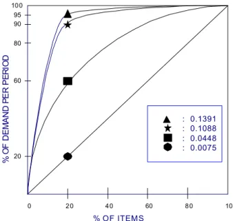
cost to holding cost of item i. As in Hausman et al. (1976) and Lee (1999, 2001), we represent the demand rate of each item as the following geometric function:

d

i = D0

p(1-p)

^i-1/(1-(1-p))ⁿ, i=1, …, n

where D0 and p are the total demand per period for all items measured in full pallet loads and the skewness parameter of the distribution, respectively. <Figure 1> shows different skewness parameters used in this experiment.

The experimental condition under which a set of example problems was solved is given as follows:

n=100; D

0

= 50000; _ξ

_i

= for all i;

α0

=0.01, 0.1, 0.2, 0.3, 0.5; p

= 0.0075, 0.0448, 0.1088, 0.1391;

S = 6; T= 6; fo

i

, i=1, …, 5 = 100, 800, 1350, 1700, 1870; O

i

, i=1, …, 6 = 0, 300, 800, 1200, 1400, 50000;

so

i

, i=1, …, 5 = 2, 1, 0.75, 0.6, 0.5; fl

i

, i=1, …, 5 = 200, 210, 222, 250, 400;

L

i

, i=1, …, 6 = 0, 20, 50, 80, 200, 50000; sl

i

, …, i=1, …, 5 = 0.4, 0.35, 0.3, 0.2, 0.1.

Note that for the definitions of the above parameters readers are referred to Section 3.

Conventionally, for the determination of storage capacity under RAN, rules of thumb have been used. One of them (here, we call it RAN1) is to set the capacity equal to 85% of that required for the FULL policy with α0= 0 (Francis et al., 1992). The overall results including those obtained by RAN1 are summarized in <Table 1> and <Table 2>. <Table 1> lists the optimal owned and leased storage capacities for α0 = 0.3 and different values of p. In the Table, α^* denotes the optimal value of for RAN.

From <Table 1>, it is observed that the owned storage capacities for RAN1 are much larger than those for RAN, which indicates that warehouses designed based on the rule of thumb are significantly larger than actually required. Relative ratios of owned storage space to the corresponding value of RAN1 given in <Table 2> come out to be around only 80%.

Also, the ratio of leased space to owned space, E/S, in

<Table 1> becomes larger as the value of p increases. This implies that as the skewness of the demand rate distribution becomes greater, larger amount of leased space relative to that of owned space is needed.

Throughput of the warehouse system measures the performance of handling operations. It is determined by the reciprocal of the expected travel time taken by a stacker crane to store or retrieve a unit load. Bozer and White (1984) and Liu (1992) presented statistical techniques to calculate the expected time for the AS/RS. Definitely, as warehouse size increases, so does the expected travel time, which in turn degrades the level of the system throughput. Therefore, in the earlier stage of system design the trade-off between the throughput and the warehouse size needs to be carefully analyzed. <Table 2> shows that the remarkable efficiency of RAN in storage/retrieval operation can be expected for any combination of skewness parameter and service level. That is, RAN's expected travel time ratios relative to RAN1 are ranged from 61.7 to 67.2%.

% O F DEM A ND P E R PE R IO D

% OF ITEMS

: 0.1391 : 0.1088 : 0.0448 : 0.0075

0 20 40 60 80 100 90

80

60

20 95 100

Figure 1. Different skewness parameters used in the experiment.

Table 1. Optimal owned storage capacities for different

values of p when α0= 0.3.

p Owned Storage Capacity RAN (

α^*

) RAN1

Leased Storage Capacity RAN(E/S)

0.0075 0.0448 0.1088 0.1391

1,677.12 (0.124) 2,672.25 1,400.0 (0.237) 2,268.86 997.5 (0.226) 1,579.21 885.4 (0.226) 1,388.63

45.73 (0.027) 54.04 (0.039) 53.25 (0.053) 53.25 (0.06)

Table 2. Storage capacity required and expected travel

time for different combinations of service level, skewness parameter, and storage policy^*.

α

0

p Owned Storage Capacity Expected Travel Time

0.1

0.0075 0.795 0.632 0.0448 0.800 0.640 0.1088 0.814 0.662 0.1391 0.820 0.672

0.5

0.0075 0.792 0.628 0.0448 0.786 0.617 0.1088 0.795 0.632 0.1391 0.799 0.638

* Figures for each combination denote relative ratios of owned storage space and expected travel time of RAN to the corresponding values of RAN1.

5. Conclusions

The storage sizing problem under RAN is considered in this paper with the objective of minimizing the overall cost of owning the storage space for the warehouse and contracting space outside of the company for shortage space. We formulate the problem as a single-variable optimization model. Optimal solutions of the model can be easily obtained by taking advantage of the convexity property for the objective function.

Using the model, we can get reasonable ideas of in-plant warehouse capacity and outsourcing storage-space amount.

The ideas should be fundamental information for a first-cut design of the starting node in a supply chain being constructed for a manufacturing company.

References

Ballou, R. H. (1999), Business Logistics Management, 4-th Ed., Prentice Hall, New Jersey, USA.

Bazaraa, M. S., Sherali, H. D., and Shetty, C. M. (1993),

Nonlinear programming: Theory and algorithms, John

Wiley & Sons, New York.

Bozer, Y. A. and White, J. A. (1984), Travel Time Models for Automated Storage/Retrieval Systems, IIE Transactions,

16(4), 329-338.

Chen, F. Y., Hum, S. H., and Sun, J. (2001), Analysis of Third-Party Warehousing Contracts with Commitments,

European Journal of Operational Research, 131,

603-610.

Cormier, G. and Gunn, E. A. (1992), A Review of Warehouse Models, European Journal of Operational

Research, 58(1), 3-13.

Cormier, G. and Gunn, E. A. (1996a), On Coordinating Warehouse Sizing, Leasing and Inventory Policy, IIE

Transactions, 28(2), 149-154.

Cormier, G. and Gunn, E. A. (1996b), Simple Models and Insights for Warehousing Sizing. Journal of the

Operational Research Society, 47(5), 149-154.

Francis, R. L., McGinnis, L. F. Jr., and White, J. A. (1992),

Facility Layout and Location: An Analytical Approach,

Prentice Hall, New Jersey, USA.

Hausman, W. H., Schwarz, L. B., and Graves, S. C. (1976), Optimal Storage Assignments in Automated Warehousing Systems, Management Science, 22(6), 629-638.

Hung, M. S. and Fisk, C. J. (1984), Economic Sizing of Warehouses- a Linear Programming Approach, Computers

and Operations Research, 11(1), 13-18.

Jucker, J. V., Carlson, R. C., and Kropp, D. H. (1982), The Simultaneous Determination of Plant and Leased Warehouse Capacities for a Firm Facing Uncertain Demand in Several Regions, IIE Transactions, 14(2), 99-108.

Lee, M.-K. (1999), Optimal Storage Capacity under Random Storage Assignment and Class-based Assignment Storage Policies, Journal of the Korean Institute of Industrial

Engineers, 25(2), 79-89.

Lee, M.-K. (2001), Warehouse Storage Capacity with Leased Space for Different Storage Policies, Journal of the

Korean Institute of Industrial Engineers, 27(4), 328-336.

Liu, F. F. (1992), Travel Time Models for Partitioning Block-and L-shaped Storage Zones for AS/RS, Proceedings

of the International Material Handling Research Colloquium,

Milwaukee, Wisconsin, 283-302.

Lowe, T. J., Francis, R. L., and Reinhardt, E. W. (1979), A Greedy Network Flow Algorithm for a Warehouse Leasing Problems, AIIE Transactions, 11(3), 170-182.

Page, E. and Paul, R. J. (1976), Multi-Product Inventory Situations with One Restrictions, Operational Research

Quarterly, 27, 15-834.

Rao, A. K. and Rao, M. R. (1998), Solution Procedures for Sizing of Warehouses, European Journal of Operational

Research, 108(1), 16-25.

Roll, Y., Rosenblatt, M. J., and Kadosh, D. (1989), Determining the Size of Warehouse Container, International Journal of

Production Research, 27(10), 1693-1704.

Rosenblatt, M. J. and Roll Y. (1988), Warehouse Capacity in a Stochastic Environment, International Journal of

Production Research, 26(12), 1847-1851.

Rosenblatt, M. J. and Roll, Y. (1984), Warehouse Design with Storage Policy Considerations, International Journal

of Production Research, 22(5), 809-821.

White, J. A. and Francis, R. L. (1971), Normative Models for Some Warehouse Sizing Problems, AIIE Transactions,

9(3), 185-190.

Zhou, G., Min, H., and Gen, M. (2001), The Allocation of Customers to Capacitated Primary and Secondary Warehouses:

Genetic Algorithm Approach, Working paper series,No.

2001-9, Logistics and Distribution Institute, Univ. of Louisville, USA.