Forest Canopy Density Estimation Using Airborne Hyperspectral Data

1. Introduction

Forest biomass is a quantity of the vegetation mass per unit area and is basic characteristic related to productivity and ecosystem processes of forest (Bonner, 1985). Forest biomass is getting important issue to climate change as forest becomes a key factor which reduces carbon dioxide of atmosphere as a

carbon sink. Forest biomass is an important indicator of carbon stocks that will help determine the contribution of forest to global carbon cycle (Kurz and Apps, 1999). Monitoring of biomass changes in forest regarded important part of monitoring carbon dioxide cycle in forest. Therefore, needs of methodologies and studies for precise estimation of forest biomass is on the rise (Shen et al., 2008).

Forest Canopy Density Estimation Using Airborne Hyperspectral Data

Tae-Hyub Kwon*, Woo-Kyun Lee**

, Doo-Ahn Kwak**, Taejin Park**, Jong Yoel Lee**, Suk Young Hong*, Cui Guishan** and So Ra Kim**

*National Academy of Agricultural Science, Rural Development Administration

**Department of Environmental Science and Ecological Engineering, Korea University

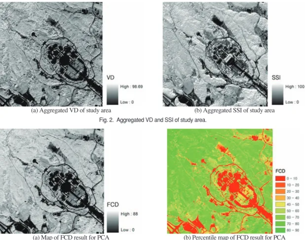
Abstract : This study was performed to estimate forest canopy density (FCD) using airborne hyperspectral data acquired in the Independence Hall of Korea in central Korea. The airborne hyperspectral data were obtained with 36 narrow spectrum ranges of visible (Red, Green, and Blue) and near infrared spectrum (NIR) scope. The FCD mapping model developed by the International Tropical Timber Organization (ITTO) uses vegetation index (VI), bare soil index (BI), shadow index (SI), and temperature index (TI) for estimating FCD. Vegetation density (VD) was calculated through the integration of VI and BI, and scaled shadow index (SSI) was extracted from SI after the detection of black soil by TI. Finally, the FCD was estimated with VD and SSI. For the estimation of FCD in this study, VI and SI were extracted from hyperspectral data. But BI and TI were not available from hyperspectral data. Hyperspectral data makes the numerous combination of each band for calculating VI and SI. Therefore, the principal component analysis (PCA) was performed to find which band combinations are explanatory. This study showed that forest canopy density can be efficiently estimated with the help of airborne hyperspectral data. Our result showed that most forest area had 60 ~ 80% canopy density. On the other hand, there was little area of 10 ~ 20%

canopy density forest.

Key Words : Airborne hyperspectral data, Forest canopy density, Remote sensing, Forest inventory, Principal Component Analysis

Received May 9, 2012; Revised June 9, 2012; Accepted June 10, 2012.

†

Corresponding Author: Woo-Kyun Lee (leewk@korea.ac.kr)

The quantification of forest volume is regarded as major forest physiognomic property (Nandy et al., 2003). Forest density is one of the most useful parameters in the planning and implementation of afforestation and reforestation program as tracking canopy density variation to monitor forestation activities as well as transformation of forest conditions over time including degradation and deforestation (Rikimaru et al., 2002).

However, field survey is time-consuming and labor-intensive work (Makela and Pekkarinen, 2004).

One of alternatives is remote sensing (RS) technique which is a nondestructive forest inventory method.

Acquisition and analysis of remotely sensed data are time-saving and cost-effective than field measurement. Furthermore, it is efficient to obtain data which are changed continuously. To estimate forest density with RS data, physically based models and fuzzy logic have been studied. But these are not suitable for large forest areas (Baret et al., 1995;

Maselli et al., 1995).

Forest canopy density (FCD) mapping program was developed by International Tropical Timber Organization (ITTO). FCD indicates the biophysical phenomenon of forests and analyzes the degree of forest density in percentage expression (Rikimaru et al., 2002). FCD mapping model presents more accurate and quantitative forest stock than forest type map expressed with high, medium, and low(Saei jamalabad and Abkar, 2004; Azizia et al., 2008).

Result of this model usually has more accuracy than other method for classify the forest density (Chandrashekhar et al., 2005; Joshi et al., 2006).

The FCD mapping model uses Landsat data which has 30 m spatial resolution for band 1~6, and 60 m for thermal band, which have up to 200 nm spectral resolution. This attribute of relatively low-spectral resolution normalizes and ignores characteristics of canopy density information of large area due to the

mixture of spectral value of various objects in one cell. Therefore, the canopy density model using low spatial- and spectral-resolution images is not very suitable for small scale forest, and has less accuracy than visual interpretation of imagery (Chandrashekhar et al., 2005).

In contrast, hyperspectral image has many bands and narrow spectral range than multispectral image such as Landsat TM. In particular, airborne hyperspectral data has generally high spatial resolution. Therefore, forest parameters which are extracted from airborne hyperspectral image usually have the improved accuracy and well represent status of forest (Sritakae, 2006). Also, it is possible to calculate forest indices through various combinations of bands with hyperspectral data. For example, normalized difference vegetation index (NDVI) can be estimated with numerous cases of narrow spectral range. Such precise NDVI can be more effective than that from wide interval band, so that it can bring more accurate results for explaining forest condition (Schlerf, 2005; Mohd Shafri et al., 2006).

Nevertheless, the application of airborne hyperspectral data for the estimation of forest parameter is still in the early stage (Sritakae, 2006).

Particularly, the estimation of forest canopy density using airborne hyperspectral data is not studied in Korea so far. In this study, we examined the possibility for estimating the forest density with the application of airborne hyperspectral data to FCD model.

2. Materials and Methods

1) Study area and data

Study area of this study is surrounding region

(around 2.0 km

) of the Independence Hall of Korea

in Cheonan city, Chungcheongnam do (Fig. 1). The forest area is composed of mainly Pinus Koraiensis (Korean pine) and Querqus spp. (Oaks).

Airborne hyperspectral data acquired at October, 2010 with CASI-1500 hyperspectral sensor with airplane. The flight was performed in October 2010 at an altitude of 1,400 m. Spectral range of CASI-1500 is 380 nm ~ 1,050 nm with up to 288 bands of which each interval is 2.4 nm ~ 19.2 nm. Also, it has 1,500 pixels across field of view (FOV) 40˚ (Heo et al., 2011). This airborne hyperspectral data has 9.6 nm spectral resolution and 0.5 m spatial resolution which has 36 bands.

FCD model for canopy density was prepared with Imagine 9.1 of Erdas Inc., ENVI 4.7 of ITT Visual Information Solutions, SAS 9.2 of SAS Institute Inc., and Visual FORTRAN of Microsoft.

(1) Forest canopy density model

FCD mapping model uses four indices such as advanced vegetation index (AVI), bare soil index (BI), shadow index (SI), and thermal index (TI).

The vegetation index (VI) responds to vegetation characteristic such as the structure and density of forest (Gitelson, 2004). In the FCD model, AVI, which is more sensitive to chlorophyll-a than NDVI (Gobron et al., 2000), was used as VI (eq.1-2).

B4 _ B3<0, AVI = 0 (1) B4 _ B3<0, AVI =

((B4 + 1)×(256 _ B3)×(B4 _ B3))

(2) Where, B3 and B4 mean Band 3 and 4 data of Landsat TM.

For more accurate calculation of the vegetation status, a bare soil index (BI), which is formulated with medium infrared range, is employed. BI increases when ground is exposed (eq.3).

BI = ×100+100 (3)

(0 < BI <200)

Where, B1 to B5 mean Band 1 to 5 data of Landsat TM.

Shadow index (SI) is defined as the ratio of shadow (eq.4). Although shadow of objects in remotely sensed data is unavoidable, it can be an useful index to estimate three dimensional structures (Ono et al., 2010). SI is related with the extraction of the low radiance in visible spectrum (Rikimaru et al., 2002).

SI = ((256 _ B1)×(256 _ B2)×(256 _ B3))

(4) Where, B1 to B3 mean Band 1 to 3 data of Landsat TM.

Not only usage of spectrum values, but also thermal information of shadow is used in FCD model (eq.5). Thermal index (TI) can be used to discriminate the black soil with high temperature and

(B5 + B3) _ (B4 + B1)

(B5 + B3) + (B4 + B1)

Fig. 1. Study area and airborne hyperspectral image.

shadow by low temperature, even if both areas have low SI value (Rikimaru et al., 2002).

The FCD can be estimated with the average integration of the vegetation density (VD) and scaled shadow index (SSI) as shown in below (Rikimaru et al., 2002).

FCD = (VD + SSI + 1)

_ 1 (5) VD is extracted by integrating VI and BI through principal component analysis (PCA). VD estimates percentile scale from bare land to high vegetation density. SSI is obtained by linear transformation of AVI and SI after black soil detection with TI and SI (Saei jamalabad and Abkar, 2004).

(2) Application of hyperspectral data to FCD model The spectral range of each Landsat TM band and corresponding hyperspectral band are shown in Table 2. Middle infrared band of Landsat TM for calculating BI and band 6 (thermal band) of Landsat TM for TI are not available in hyperspectral data (Table 1). Therefore, it is impossible to extract two indices of BI and TI directly from hyperspectral data.

Theoretically, TI can be used to discriminate black soil and forest shadow, while BI represents the bare land. There appears rarely bare soil area in study site, so the distinction of black soil and forest shadow does not be needed further. Therefore, the canopy density can be calculated just with VI and SI.

According to formulation AVI, hyperspectral bands were combined to 40 cases with 4 red bands

and 10 NIR hyperspectral bands. SI formulated with red, green, and blue bands of hyperspectral data had 64 combinations. Using these combinations of AVI and SI, the normalization was performed to calculate VD and SSI with following equation (eq.6):

nomalization = ×100 (6)

Where, ‘min’ means minimum value of each index and ‘max’ means maximum value of each index.

The FCD is estimated in cases of 2,540 with 40 cases of VD and 64 cases of SSI. Because of many combinations of FCD, VD and SSI were analyzed in PCA analysis to integrate all band combinations by the weight of given eigenvalue and eigenvector. After PCA process, each representative of VD and SSI was calculated, and then computed to FCD.

To assess the accuracy of FCD results, canopy volume to entire vegetation volume in unit area was measured in field survey. Because hyperspectral data have high resolution enough to detect individual trees, each plot for volume measurement was set to 1 m

. 67 plots with 1 m x 1 m were randomly selected, and tree height and crown base height were measured. Finally, the rates of canopy volume to vegetation volume were compared with mean FCD.

(3) Index integration with PCA

One of the most important problems of hyperspectral data is the massively large and high data dimensionality. PCA is a popular tool for reducing the dimensionality of hyperspectral data that

value _ min max _ min Table 1. Hyperspectral bands and corresponding Landsat TM bands

Landsat TM Band Spectrum(mm) Hyperspectral bands

1 Blue 0.45 - 0.52 5, 6, 7, 8

2 Green 0.52 - 0.60 10, 11, 12, 13

3 Red 0.63 - 0.69 15, 16, 17, 18

4 Near infrared 0.76 - 0.90 21, 22, 23, 24, 25, 26, 27, 28, 29, 30

5 Middle infrared 1.55 - 1.75 -

6 Thermal infrared 10.4 - 12.5 -

Landsat TM Band Spectrum(mm) Hyperspectral bands

represent most of the information presented in the original image, and for identifying optimal bands related with interesting area (Tsai et al., 2007;

Torbick and Becker, 2009).

PCA is a mathematical process that uses a perpendicular transformation to convert a set of correlated observations into a set of values of uncorrelated variables called principal components.

In transformation, the first principal component has the highest variance, and succeeding components have lower values in turn (Jolliffe, 2002).

Therefore, one representative FCD image was prepared as implying all characteristics of band combinations through the PCA process. In the PCA procedure, eigenvalues and eigenvectors are calculated from covariance matrix. Eigenvalue shows how much the component is correlated with the original image, and can be an explanatory value.

Eigenvector is the matrix of the values which is multiplied with each band to calculate eigenvalue.

In this study, eigenvalues and eigenvectors were calculated from each result of VD and SSI.

Thereafter, the ratios of absolute values in each eigenvectors were calculated and multiplied with the corresponding ratios of each component’s eigenvalues. All ratios to each combination were summed and considered as weights of combinations.

Weights were multiplied to each combination, and then these combinations were integrated. Finally, representative VD and SSI were generated.

3. Results and Discussion 1) Index combinations

(1) AVI and VD

40 cases of AVIs were calculated from the combination of red and NIR in hyperspectral bands.

As the result, buildings, paved area and grassland

area showed low value in AVI. With AVI results, the normalization of each cell value was progressed to calculate VD. In particular, some results showed low vegetation index of grass land around buildings with very black color. Combinations with red spectrum, which are closer to band 30, had higher mean values of vegetation density. It can imply that the reflection on vegetation was the most sensitive in the red spectrum, long wavelength.

(2) SI and SSI

As the same conceptual work with AVI and VD calculation, SI combinations with red, green, and blue bands were calculated to 64 cases. All SIs had range of 1 to 256. A high SI value means a high value of red, green, and blue spectral value, so that such area looked like black. The SI combinations are normalized to SSI. In the SSI results, roads and paved area showed very low values whereas forest areas show high. Overall color scheme was not different each other, but SSIs combined with long wavelength spectrum in red range usually showed high.

2) FCD estimation by PCA (1) PCA process of VD and SSI

VDs were integrated to one representative VD after each weight given. In order to calculate each weight of VD, PCA was performed with ENVI 4.7.

In the result of VD 1 ~ 40, component 1 shows significantly high eigenvalue with 97.33% of total eigenvalue. Moreover, eigenvalue rapidly decrease when component increase. At the component 7, the accumulated eigenvalue rate was over 99.99%. This means that 99.99% of VDs can be explained within component from 1 to 7. With these eigenvalues and corresponding eigenvector, every weight of each VD extracted.

VD 6 was analyzed as the most effective

representative from band combination with weight of

0.32405, and VD 3 was followed with weight of 0.13368. The VD 38 had 0.00008 weight, which is lowest. All of weights were multiplied with corresponding VDs, and then stacked into one VD.

The integrated VD was converted to an image as shown in Fig. 2.

The VD range from 0 to 98.69 and black colored area, which is 0 of VD value, is shown at paved area and buildings, whereas northern west and southern east area are displayed with high rate.

The PCA result of SSI indicates that component 1 had 99.67% of whole eigenvalue and component 2 had 0.21% of all eigenvalue. Especially, subsequent components of component 48 had 0 eigenvalues and the sum of component 1 ~ 3 had 99.9% of accrued

eigenvalue. Finally, SSI 38 had the highest weight although the deviation of weights between each SSI was not so large in contrast with VDs. The consequence of integrating weighted SSIs is shown in Fig. 2.

Integrated SSI showed low value at road and paved area as well as grassland. However, northwest and southeast area where show high VD had the high level of SSI.

(3) PCA result of FCD

By the equation of FCD, comprehensive VD and SSI through PCA were combined to a FCD result and shown in Fig. 3.

FCD has the range over 88% of canopy density, and particularly shows high in the area where show Fig. 2. Aggregated VD and SSI of study area.

(a) Aggregated VD of study area (b) Aggregated SSI of study area

Fig. 3. FCD result maps.

(a) Map of FCD result for PCA (b) Percentile map of FCD result for PCA

high in VD and SSI. In the FCD map, roads and paved area clearly showed 0 values, and the grass land had low level of FCD. Based on this FCD map, percentile map is depicted in Fig. 3.

In the percentile map, the medium density displayed with yellow color can be easily distinguished from the high density with green color in forest area.

In the study area, forest area usually has high density while low density forest appears in roads and paved area. Moreover, 70 ~ 80% forest density occupies the largest area (612,560 m

), and 60 ~70% density showed 526,130 m

. These two ranges occupy 65%

of whole forest area. 10 ~ 20%, 20 ~ 30%, and 80 ~ 90% canopy density were less than 50,000 m

in this study, and three density occupied only 5% of all forest area (Table 2).

To assess the accuracy of this FCD result, the correlation analysis was performed with field- surveyed data (Fig. 4).

Given 0.34 of R

and 5.70 of RMSE in correlation analysis, the accuracy of FCD result was relatively low. That’s why 13 plots of filed-survey data had overestimated measures in 60 ~ 70% density range.

In particular, most of overestimated plots were broad

leaf stand. It is attributed to the difference of leaf area and density by tree species.

4. Conclusion

This study presents an estimation of forest canopy density in the Independence Hall of Korea area from airborne hyperspectral data with the help of Forest Canopy Density (FCD) mapping model investigated by International Tropical Timber Organization (ITTO). Parameters used in FCD mapping model are vegetation index (VI), Bare soil index (BI), shadow index (SI), and thermal index (TI). In this study, only VI and SI are used for estimating FCD. BI by Landsat TM middle infrared spectrum and TI by Landsat TM thermal band could not be drived with airborne hyperspectral data due to spectral scope differences. Vegetation density (VD) presenting a continuing range from bare land to high vegetation, and scaled shadow index (SSI) were combined to numerous cases. These results were grouped into some clusters through the cluster analysis. Also, these VDs and SSIs were integrated into single VD and SSI image with PCA process. And then, they are synthesized to FCD output.

As the result, study site has 60 ~ 80% of forest canopy density in most forest area. And this result was compared with the field data inquired into the in- situ plot of study site. Overall accuracy of the result showed especially overestimation in 60 ~ 70% of actual density range. It is attributed to the large area of broad leaf trees and leaf density. Even if its accuracy was low with field survey data, its correlation with physiological phenomenon and Fig. 4. Correlation of field data and FCD result for PCA.

Table 2. Area of each percentage in FCD results

Percentile 0~10 10~20 20~30 30~40 40~50 50~60 60~70 70~80 80~90

Area (ha) 25.21 1.80 4.20 8.04 15.19 28.48 52.61 61.26 3.29

Rate (%) 12.60 0.90 2.10 4.02 7.59 14.23 26.30 30.62 1.64

Percentile 0~10 10~20 20~30 30~40 40~50 50~60 60~70 70~80 80~90

applications of indices using narrow spectrum bands from hyperspectral data are useful for forest density estimation with RS technique as a tool of measurement.

Forest canopy density reveals the actual forest status and is considered as an important parameter related to forest management. Forest canopy density is also closely related to forest stock and biomass.

With multi temporal analysis using time series data of FCD, forest monitoring and land-cover change detection are possible.

Acknowledgment

This study was carried out with the support of

‘Forest Science & Technology Projects (Project No.

S210912L010100) provided by Korea Forest Service.

References

Azizia, Z., A. Najafi, and H. Sohrabia, 2008. Forest Canopy Density Estimating Using Satellite Images, Proc. of The International Society for Photogrammetry and Remote Sensing Congress Commission VIII, Beijing, China, July 3-11, XXXVII. Part B8.

Baret, F.J., G.P.W. Clevers, and M.D. Steven, 1995.

The robustness of canopy gap fraction estimates from red and near-infrared reflectances: a comparison of approaches, Remote Sensing of Environment, 54(2): 141- 151.

Bonner, G.M., 1985. Inventory of forest biomass in Canada, Petawawa National Forestry Institute, Canadian Forest Service.

Chandrashekhar, M.B., S. Saran, P.L.N. Raju, and P.S. Roy, 2005. Forest Canopy Density

Stratification: How Relevant is Biophysical Spectral Response Modelling Approach?, Geocarto International, 20(1): 15-21.

Gitelson, A.A., 2004. Wide Dynamic Range Vegetation Index for Remote Quantification of Biophysical Characteristics of Vegetation, Journal of Plant Physiology, 161(2): 165-173.

Gobron, N., B. Pinty, M.M. Verstraete, and J.L.

Widlowski, 2000. Advanced Vegetation Indices Optimized for Up-Coming Sensors:

Design, Performance, and Applications, IEEE Transactions on Geoscience and Remote Sensing, 38(6): 2489-2505.

Heo, H.S., S.H. Kim, H. Lee, K.J. We, Y.R. Park, and S.Y. Cho, 2011. A study of Forest Species Classification using Airborne Hyperspectral Imagery, Proc. of the Korean Society of Remote Sensing Spring Conference 2011, Kyoung-Ju, Korea, March 24-25, pp. 290-295.

Jolliffe, I.T., 2002. Principal Component Analysis, Springer-Verlag, New-York.

Joshi, C., J.D. Leeuw, A.K. Skidmore, I.C. Duren, and H. Oosten, 2006. Remotely sensed estimation of forest canopy density: A comparison of the performance of four methods, International Journal of Applied Earth Observation and Geoinformation, 8: 84-95.

Kurz, W.A. and M.J. Apps, 1999. A 70-Year Retrospective Analysis of Carbon Fluxes in the Canadian Forest Sector, Ecological Applications, 9(2): 526-547.

Makela, H. and A. Pekkarinen, 2004. Estimation of forest stand volumes by Landsat TM imagery and stand-level field-inventory data, Forest Ecology and Management, 196: 245-255.

Maselli, F., C., Conese, T.D. Filippis, and S. Norcini,

1995. Estimation of forest parameters through

fuzzy classification of TM data, IEEE

Transactions on Geoscience and Remote

Sensing, 33(1): 77-84.

Mohd Shafri, H.Z., M.A. Mohd Salleh, and A.

Ghiyamat, 2006. Hyperspectral Remote Sensing of Vegetation Using Red Edge Position Techniques, American Journal of Applied Sciences, 3(6):1864-1871.

Nandy, S., P.K.. Joshi, and K.K. Das, 2003. Forest Canopy Density Stratification Using Biophysical Modeling, Journal of the Indian Society of Remote Sensing, 31(4):291-297.

Ono, A., K., Kajiwara, and Y. Honda, 2010.

Development of new vegetation indexes, shadow index (SI) and water stress trend (WST), Proc. of International Society for Photogrammetry and Remote Sensing Technical commission VIII Symposium, Kyoto, Japan, August 9-12, XXXVIII, Part 8.

Rikimaru, A., P.S. Roy, and S. Miyatake, 2002.

Tropical forest cover density mapping, Tropical Ecology, 43(1):39-47.

Saei jamalabad, M. and A.A. Abkar, 2004. Forest Canopy Density Monitoring Using Satellite Images, Proc. of The International Society for Photogrammetry and Remote Sensing Congress, Istanbul, Turkey, July 12-23, XXXV.

Schlerf, M., C. Atzberger, and J. Hill, 2005. Remote sensing of forest biophysical variables using HyMap imaging spectrometer data, Remote Sensing of Environment, 95: 177-194.

Shen, M., Y. Tang, J. Klein, P. Zhang, S. Gu, A.

Shimono, and J. Chen, 2008. Estimation of aboveground biomass using in situ hyperspectral measurements in five major grassland ecosystems on the Tibetan Plateau, Journal of Plant Ecology, 1(4): 247-257.

Sritakae, A., 2006. Predictive relations of forest stand parameters from hyperspectral remote sensing at Thetford Forest, the UK. Enschede, ITC Torbick, N. and B. Becker, 2009. Evaluating

Principal Components Analysis for Identifying Optimal Bands Using Wetland Hyperspectral Measurements From the Great Lakes, USA, Remote Sensing, 1(3):408-417.

Tsai, F., E.K. Lin, and K.Yoshino, 2007. Spectrally

segmented principal component analysis

hyperspectral imagery mapping invasive plant

species, International Journal of Remote

Sensing, 28(5):1023-1039.