딥러닝 사물 인식 알고리즘(YOLOv3)을 이용한 미세조류 인식 연구
박정수1⋅백지원2a⋅유광태2b⋅남승원3⋅김종락2c,†
1
국립한밭대학교 건설환경공학과⋅
2(주)유앤유⋅
3국립낙동강생물자원관 원생생물연구팀
Microalgae Detection Using a Deep Learning Object Detection Algorithm, YOLOv3
Jungsu Park1⋅Jiwon Baek2a⋅Kwangtae You2b⋅Seung Won Nam3⋅Jongrack Kim2c,†
1
Dept. of Civil & Environmental Eng., Hanbat National University
2
UnU Inc.
3
Protist Research Team, Nakdonggang National Institute of Biological Resources
(Received 11 May 2021, Revised 20 June 2021, Accepted 14 July 2021)
Abstract
Algal bloom is an important issue in maintaining the safety of the drinking water supply system. Fast detection and classification of algae images are essential for the management of algal blooms. Conventional visual identification using a microscope is a labor-intensive and time-consuming method that often requires several hours to several days in order to obtain analysis results from field water samples. In recent decades, various deep learning algorithms have been developed and widely used in object detection studies. YOLO is a state-of-the-art deep learning algorithm. In this study the third version of the YOLO algorithm, namely, YOLOv3, was used to develop an algae image detection model. YOLOv3 is one of the most representative one-stage object detection algorithms with faster inference time, which is an important benefit of YOLO. A total of 1,114 algae images for 30 genera collected by microscope were used to develop the YOLOv3 algae image detection model. The algae images were divided into four groups with five, 10, 20, and 30 genera for training and testing the model. The mean average precision (mAP) was 81, 70, 52, and 41 for data sets with five, 10, 20, and 30 genera, respectively. The precision was higher than 0.8 for all four image groups. These results show the practical applicability of the deep learning algorithm, YOLOv3, for algae image detection.
Key words : Deep learning, Microalgae, Object detection, Water supply system, YOLOv3
1조교수(Assistant Professor), [email protected], https://orcid.org/0000-0002-9780-6988
2a선임(Junior Engineer), [email protected], https://orcid.org/0000-0003-4407-6085
2b대표이사(CEO), [email protected], https://orcid.org/0000-0002-3735-2312
3전임연구원(Associate Researcher), [email protected], https://orcid.org/0000-0002-8722-5223
2c,†Corresponding author, 수석(Principal Engineer), [email protected], https://orcid.org/0000-0001-5163-6146
This is an Open-Access article distributed under the terms of the Creative Commons Attribution Non-Commercial License (http://creativecommons.org/
licenses/by-nc/3.0) which permits unrestricted non-commercial use, distribution, and reproduction in any medium, provided the original work is properly cited.
1. Introduction
Algal bloom is one of the important issues in the management of drinking water supply systems. The overgrowth of algae has various harmful effects on water quality such as unfavorable odor or taste (Codd et al., 2005;
Paerl and Otten, 2013; WHO, 2004). The cell walls of diatoms are not removed by the regular disinfection process and often cause technical problems such as clogging of filtration beds in water treatment plants. Cyanobacteria release algal toxins in freshwater systems, which cause direct damage to human health.
Thus, continuous monitoring of algae in freshwater such as rivers and reservoirs is essential. One of the most common and traditional monitoring methods is the visual identification of algae using a microscope. However, this is laborious and time-consuming. Thus, the development of a rapid and less labor-intensive method for algae image identification is required.
Object detection is a fundamental subject and is continuously studied in computer vision research (Zhao et al., 2019). Object detection technology based on deep learning algorithms has made noticeable accomplishments in recent decades. The convolutional neural network (CNN) is the most representative and widely used deep learning algorithm in object detection studies (LeCun et al., 2015;
Zhao et al., 2019). The characteristics of the target image are extracted by computation processes called convolution and pooling and used for the classification of the target object. AlexNet, a deep learning algorithm based on the convolutional neural network, was a winner in the 2012 image net large scale visual recognition challenge (ILSVRC) and is considered one of the algorithms that shows the practical applicability of deep learning in object detection (Krizhevsky et al., 2012; Russakovsky et al., 2015). Since AlexNet, various algorithms have been developed, and these models can be categorized into two types (i.e., one-stage model and two-stage model)(Sultana et al., 2020; Zhao et al., 2019).
Regions with convolutional neural network (R-CNN) is one of the first two-stage object detection models developed.
In the first stage of R-CNN, the algorithm proposes multiple possible regions where a target object can be located. In the second stage, the model finds the location of the target object and classifies it using the CNN algorithm (Girshick et al., 2014; Zhao et al., 2019). Various two-stage object detection algorithms that have improved on R-CNN have been developed, such as spatial pyramid pooling (SPP), Fast R-CNN, Faster R-CNN, and Mask R-CNN(Girshick, 2015;
He et al., 2017; He et al., 2015; Ren et al., 2015).
YOLO is considered one of the most representative one-stage object detection models where the region proposal and classification are unified and processed in a single stage (Redmon et al., 2016; Sultana et al., 2020). There are also various one-stage object detection models such as single shot multibox detector (SSD) and Retina-Net (Lin et al., 2017;
Liu et al., 2016). The YOLO model was continuously improved from version 1 to version 3, and Redmon and Farhadi (2018) proposed a third version of the YOLO model(YOLOv3). The inference time of YOLOv3 for object detection process ranges from 22 to 51 milliseconds depending on the resolution of input images, which is a much faster inference time than other models such as SSD and RetinaNet (Redmon and Farhadi, 2018). Although YOLOv3 has slightly less accuracy than these two models, the noticeably faster inference time can be considered one important advantage of the YOLO model as a real-time object detection model (Redmon and Farhadi, 2018). Object detection model development is a competitive field and there are still various ongoing issues. Thus, it is the researcher’s choice to select an optimal model for their research field.
Recently, several studies present the practical possibility of using deep learning models such as YOLO for algae image detection (Pedraza et al., 2018; Salido et al., 2020). Pedraza et al. (2018) used the YOLO model for the classification of diatoms, and it classified objects of nine diatom species in images with overall precision and recall of 0.74. More recently, Salido et al. (2020) used YOLO to classify 10 diatom species with mean precision of 0.727. The composition of the input image data set such as the number of target objects and use of colors affect the object model performance while related research in algal image detection is still in an early stage.
In this study, a deep learning object detection algorithm, YOLOv3, was used for the detection and classification of algae images obtained from freshwater. The model was trained and tested for the classification of five, 10, 20, and 30 target species so that the effect of the number of target objects on model performance could be analyzed and the practical applicability of the model verified, where the effect of color of the images on model performance was also compared using the same data groups with grayscale photos.
2. Materials and Methods
2.1 Data sources
2.1.1 Image acquisition
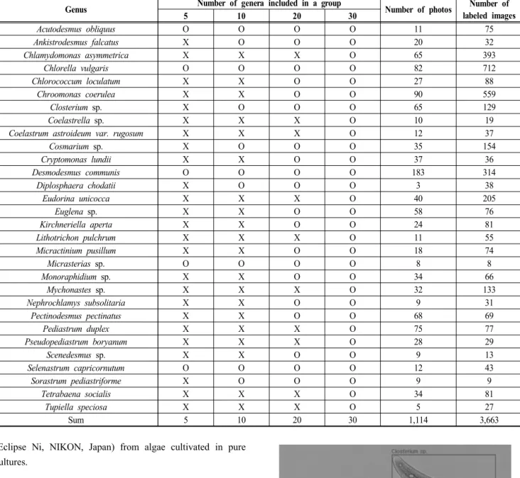
A total of 1,114 photos with 3,663 objects for 30 genera
were used to develop the YOLOv3 algae image detection
model (Table 1). The photos were collected by microscope
(Eclipse Ni, NIKON, Japan) from algae cultivated in pure cultures.
2.1.2 Input image data set and labelling
The algae images were divided into four groups with five, 10, 20, and 30 genera (Table 1) to compare the model’s performance with various numbers of target objects for classification. The color of the images can affect model performance, especially as the number of target genera increases. Thus, each data group was also prepared with grayscale photos to test the model’s sensitivity to the colors of the algae images. Thus, the YOLOv3 model was trained with eight different data sets. The ratio of data used for model training and testing is 7:3.
Each photo contains more than one cell image object, and each algal cell image object was labeled manually for training and testing the YOLOv3 model using a labeling program developed in this study (Table 1). For example, there were 11 photos of Acutodesmus obliquus where each
photo contained from one to several cell image objects.
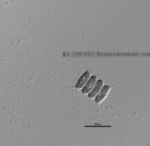
Thus, a total of 75 Acutodesmus obliquus objects were labelled. The label includes the coordinates of the bounding box and class of the target object so that the model identifies the location and class of each cell object during the training process (Fig. 1).
Fig. 1. Example of algae cell image labelling.
Genus Number of genera included in a group
Number of photos Number of labeled images
5 10 20 30
Acutodesmus obliquus O O O O 11 75
Ankistrodesmus falcatus X O O O 20 32
Chlamydomonas asymmetrica X X X O 65 393
Chlorella vulgaris O O O O 82 712
Chlorococcum loculatum X X O O 27 88
Chroomonas coerulea X X O O 90 559
Closterium sp. X O O O 65 129
Coelastrella sp. X X X O 10 19
Coelastrum astroideum var. rugosum X X X O 12 37
Cosmarium sp. X O O O 35 154
Cryptomonas lundii X X O O 37 36
Desmodesmus communis O O O O 183 314
Diplosphaera chodatii X O O O 3 38
Eudorina unicocca X X X O 40 205
Euglena sp. X X O O 58 76
Kirchneriella aperta X X O O 24 81
Lithotrichon pulchrum X X X O 11 55
Micractinium pusillum X X O O 18 74
Micrasterias sp. O O O O 8 8
Monoraphidium sp. X X O O 34 66
Mychonastes sp. X X X O 32 133
Nephrochlamys subsolitaria X X O O 9 31
Pectinodesmus pectinatus X X O O 68 69
Pediastrum duplex X X X O 75 77
Pseudopediastrum boryanum X X X O 28 29
Scenedesmus sp. X X O O 9 13
Selenastrum capricornutum O O O O 12 43
Sorastrum pediastriforme X O O O 9 9
Tetrabaena socialis X X X O 34 81
Tupiella speciosa X X X O 5 27
Sum 5 10 20 30 1,114 3,663
Table 1. Algae images used for YOLOv3 model development
2.2. Model development
2.2.1 YOLOv3 model
YOLOv3 predicts the location and class of objects in a single neural network process where a convolutional neural network with 53-layer, Darknet-53 is used as the main model network (Redmon and Farhadi, 2018). YOLOv3 has been continuously improved from YOLOv1 and YOLOv2 (Redmon et al., 2016; Redmon and Farhadi, 2017, 2018).
YOLOv1, the first version of the YOLO model, divides the input image into an S×S grid where S=7 is used to evaluate the model (Redmon et al., 2016). Each grid cell predicts B (assigned as 2) bounding boxes for object detection and the confidence score is calculated for each bounding box.
The confidence score is defined as P×IOU, where P is the probability that the bounding box contains an object and IOU is intersection over union (Redmon et al., 2016). IOU is calculated with the following equation (Eq. 1), as illustrated in Fig. 2.
Each bounding box contains five values. These values are coordinates (x, y) that represent the center of the box relative to the bounds of the grid, the width (w) and height (h) of the box, and the confidence score (Redmon et al., 2016). Thus, each grid prediction consists of S×S×(B×5+C) tensor where C is the number of object classes trained.
YOLOv1 is evaluated with S=7, B=2, and C=20 using the PASCAL VOC data set (Redmon et al., 2016). The bounding box with the highest IOU with ground truth is assigned as responsible for predicting an object. YOLOv2 is improved from YOLOv1. YOLOv2 uses a convolutional neural network with 19 layers, called Darknet-19, and anchor boxes to predict bounding boxes.
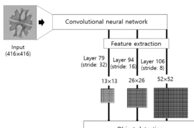
YOLOv3 has several important improvements from the previous version of YOLO models. First, YOLOv3 uses Darknet-53 as the main model network. YOLOv3 also
extracts three different scales of images, called a feature map. The size of each feature map is 13×13, 26×26 and 52×52 (Redmon and Farhadi, 2018; Zhao and Ren, 2019).
Each grid cell has three anchor boxes with different shape scores. A model structure diagram of Darknet-53 and YOLOv3 can be found in previous studies (Pedraza et al., 2018; Tian et al., 2019; Zhao and Ren, 2019), and a simple schematic is shown in this study (Fig. 3). The attributes of each anchor box are the location of object, objectness score and class (Fig. 4)(Redmon and Farhadi 2018). The objectness score is also predicted for each bounding, which represents the probability of whether the target in the bounding box is an object. Each bounding box also predicts the classes of the target object contained in the bounding box using logistic classifiers so that multilabel classification is possible (Redmon and Farhadi, 2018).
2.2.2 Model training and optimization
The eight input data sets were trained by YOLOv3 coded by C++ language. The model frame was programed by C#
language using OpenCV 4.4 and NVDIA GPU Toolkit 11.
The model was trained by Darknet YOLO (https://github.com/
AlexeyAB/darknet) where pre-trained Darknet53.conv.74 was used. The hyperparameters were used with default values of the YOLOv3 model with batch size 64, learning rate 0.001, and max_batch the number of class×2000. The best model was determined by comparing model performance for every 100 batches.
Fig. 3. Schematic of YOLOv3 structure.
Fig. 4. Attributes of a bounding box. n is the number of classes for prediction.
(1)
(a) Area of overlap (b) Area of union Fig. 2. Schematic of area of overlap and area of union for
IOU calculation.
2.3. Model evaluation
2.3.1. Precision and mean average precision
For object detection, the model prediction can be divided into four indicators as follows.
⋅True positive(TP): the number of observed positive values that were correctly predicted,
⋅False positive(FP): the number of observed positive values that were wrongly predicted,
⋅False negative(FN): the number of observed negative values that were wrongly predicted,
⋅True negative(TN): the number of observed negative values that were correctly predicted.
The model performance can be evaluated by precision(PR) and recall(RE) defined by the four indicators(Eq. 2-3).
(2)
(3)
The Precision-Recall curve (P-R curve) represents the change of PR through the change of recall over an interval from 0 to 1, which is commonly used to consider both PR and recall for object detection model evaluation (Ozenne et al., 2015; Tian et al., 2019).
The average precision (AP) is calculated from the sum of the area under the P-R curve for each class of image, representing the average of precision through the overall interval of recall. The mean average precision (mAP) is the average of AP for all image classes. Redmon and Farhadi (2018) verified that YOLOv3 performs well with an IOU of 50%, and Zhao and Ren (2019) also noted that the YOLOv3
model performs strongly with an IOU of 50%. In this study, the model performance was evaluated by PR and mAP using an IOU of 50%.
3. Results and discussion
3.1 Model performance comparison
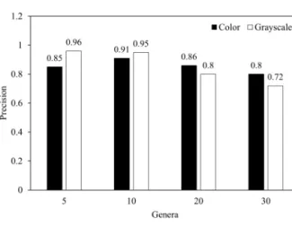
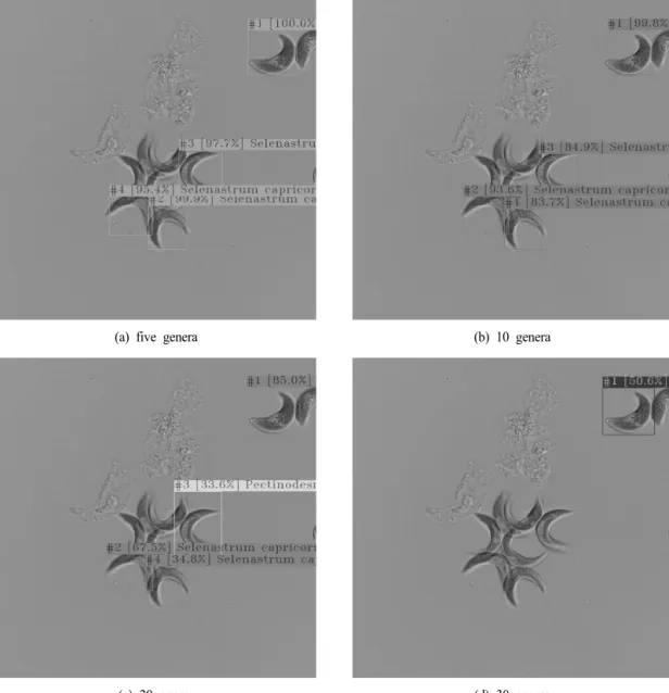
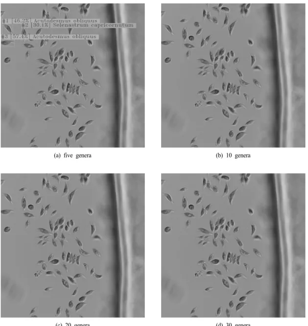
The model performance for eight data sets was compared in Fig. 5. The model shows better mAP for data sets with a small number of genera, both for color and grayscale image.
The mAP was 81, 70, 52, and 41 for data sets with five, 10, 20, and 30 genera, respectively. PR was higher than 0.8 for all data sets with color images, and the highest PR was observed for the data set with 10 genera. The model using grayscale images had about 11% and 4% higher PR for data sets with five and 10 genera, respectively, while it had about 6% and 8% lower PR for data sets with 20 and 30 genera.
The model shows better performance for data sets with a small number of genera when using grayscale images. On the other hand, higher PR was observed when using color images for data sets with a larger number of genera. These results suggest that color images provide more useful information for object detection and improve model PR when a relatively larger number of genera is classified.
3.2 Detection characteristics