EVALUATION OF TURBULENCE MODELS IN A HIGH PRESSURE TURBINE CASCADE SIMULATION

E VALUATION OF T URBULENCE M ODELS

IN A H IGH P RESSURE T URBINE C ASCADE S IMULATION

M. M. El-Gendi,

K.-U. Lee,

W. J. Chung,

C.-Y. Joh

and C. H. Son

1

School of Mechanical Engineering, Univ. of Ulsan, Ulsan, Korea

2

Mechanical Power & Energy Department, Minia Univ., Minia, Egypt

고압터빈 익렬 주위 유동해석에서 난류모델의 영향 평가

M. M. El-Gendi,

이 경 언,

정 의 준 ,

조 창 열 ,

손 창 호

1울산대학교 기계공학부

2

Mechanical Power & Energy Department, Minia Univ., Minia, Egypt

Steady flow simulations through a high pressure turbine guide vanes were carried out. The main objective of the present work is to study the performance of turbulence models on the steady flow prediction from aerodynamic and aerothermal points of view. Three turbulence models were compared, namely SST, k-ω and ω-Reynolds stress models. The laminar results were also compared. The comparison was done with emphasis on the isentropic Mach number and heat transfer coefficient along the blade, and total pressure loss in the wake region. The calculated isentropic Mach number showed reasonable agreement with experimental data along the blade surface for all three turbulent models. For the total pressure loss in the wake region, ω-Reynolds stress model showed the best agreement with the experimental data. However, unless using an appropriate transition model, the heat transfer coefficients of all three turbulent models showed poor agreement with experimental data.

Key Words : Gas turbines(가스터빈 ), CFD(전산유체역학), Turbulence model(난류모델 ), Steady flow(정상유동 ), Transonic flow(천음속유동 )

Received: May 2, 2011, Revised: August 16, 2012, Accepted: August 18, 2012.

* Corresponding author, E-mail: [email protected] DOI http://dx.doi.org/10.6112/kscfe.2012.17.3.053

Ⓒ KSCFE 2012

1. I NTRODUCTION

Flow pattern through high loaded subsonic and transonic turbine cascades is very complicated. These flows are usually combined with transition and separation along the blade surface, along with vortex shedding from the trailing edge and shock waves. Therefore, for a good blade design and a better understanding of the flow phenomena, it is important to investigate these flows through accurate numerical predictions.

Arts et al.[1] experimentally studied a high loaded turbine cascade at different flow conditions. They studied both aerodynamic and aero-thermal behavior of the subsonic and transonic flows at different Mach and Reynolds numbers and with different free stream turbulent intensities. Using these huge data of Arts et al.[1], many researchers tried to validate numerical techniques or studied the performance of various turbulence models.

Liu[2] checked the validity of a newly developed

numerical scheme (Modified Implicit Flux-Vector-Splitting)

with this flow pattern from aerodynamic view point. He

showed that this method can reasonably capture most of

the flow physics for this type of flow. Liu[3] also

validated this method from aero-thermal point of view as

well by showing good agreement with experimental data

and other published calculation results. Gehrer and

Jericha[4] studied the performance of several turbulent

different turbulence models in predicting the flow around the blade and in the wake region from aerodynamic and aero-thermal point of view. Also, the comparison will include our laminar calculation results and the steady turbulent calculation results of Liu[2,3] using low Reynolds number k-ε model

2. I NVESTIGATED CASCADE

The investigated cascade is a high pressure turbine guide vane. The blade coordinates can be found in Arts et al.[1], and the cascade dimensions are shown in Table 1.

3. N UMERICAL METHOD

3.1 C OMPUTATIONAL GRID

Fig. 1 shows the grid topology. The O-H type grid was used in all cases. The O type grid around the blade provided the good resolution and orthogonality to the blade surface. The H type grid applied in the remaining of the domain provided good resolution in the wake region and improved the skewness. Three different number of total nodes, namely about 0.66×10

, 1.24×10

, and 1.7×10

were tested and found no substantial difference to the results. However, different turbulent models can result different y+ value and we do not know this value before calculation, we chose 1.24×10

grids to be safe for all cases.

3.2 B OUNDARY CONDITIONS

We investigated two test cases in the present work:

Name Symbol Dimension Unit

chord C 67.647 mm

axial chord Cax 36.462 mm

pitch g 57.500 mm

stager angle ϒ 55.000 deg

Table 1 Dimension of Cascade

Fig. 1 Computational grid

adiabatic case and isothermal case. The isothermal boundary condition approximately represents real condition of a jet engine in which the blade is cooled by a coolant to an approximately constant temperature while the incoming flow has much higher temperature. Therefore, there exists heat transfer between the blade surface and the fluid. In this case, we treated the blade surface as isothermal surface. The adiabatic case approximately represents the case that encountered in many wind tunnel experiments in which the ambient flow temperature and the blade wall temperature has no significant difference.

Therefore, the blade is approximately insulated and we treated the blade wall as adiabatic surface. The turbine cascade of both cases in this study is the same as that used in Arts et al.[1]. All calculations for adiabatic case have the exit isentropic Mach number (M

= 1.02) and exit isentropic Reynolds number (Re

= 1.0×10

), based on chord length. On the other hand, all calculations for isothermal case (VKI MUR235) have the exit isentropic

Name Adiabatic Isothermal Inlet total Pressure, P01(kpa) 159.600 182.000 Inlet total temperature, T01(K) 415.000 413.000

Wall temperature, Tw(K) 301.150

Exit Mach number, M2,is 1.020 0.927

Table 2 Boundary Condition

Fig. 2 Mach number contour for k-ω turbulence model

Mach number (M

= 0.927) and exit isentropic Reynolds number (Re

= 1.15×10

). In this simulation, both total pressure and total temperature are imposed at the inlet boundary and static pressure is prescribed at the exit boundary(see Table 2). Also, the non-slip condition is used on the surface of the blade. In the pitch direction, periodic boundary condition is used.

3.3 Numerical schemes and convergence

Commercial CFD package, ANSYS-CFX (ANSYS, Inc, Canonsburg, PA), is used in this study. In this package, the cell vertex finite volume method is used for spatial discretization. The transient scheme is Second Order Backward Euler and a high resolution scheme[6] is used to treat the advection terms.

3.4. T URBULENT MODELS

Three turbulent models are compared in this study.

They are SST[7] model, k-ω[8] model and ω-Reynolds stress model (ω-RS[9,10]). Both SST and k-ω turbulence models are based on eddy viscosity hypothesis. On the other hand, ω-RS turbulent model is based on the transport equations for all components of Reynolds stress tensor. ω-RS turbulent model uses ω instead of the dissipation rate ε and has advantage of more accurate near wall treatment over standard Reynolds stress model. SST turbulent model combines the advantage of k-ω turbulent model near the inner region of the boundary layer and high Reynolds number version of k-ε model in the outer region. In addition, SST turbulent model accounts for the transport effects of turbulent shear stress.

3.5 C ONVERGENCE

Initially, 500 iteration is performed for the SST model and it is found that the normalized residual dropped to the

Fig. 3 Isentropic Mach number distribution along blade surface; Experiment was carried out by Arts et al.[1]

order of 10

around 200 iteration and remain essentially unchanged until 500 iteration. Additional 2500 iteration is performed but no noticeable change of residual is observed. Almost identical residual changes are observed for other cases except that the limting normalized residual dropped to a slightly larger value for ω-Reynolds stress model. Therefore we determine 500 iteration is sufficient for convergence for all cases.

4. R ESULTS AND DISCUSSION

4.1 A DIABATIC CASE

Fig. 2 shows the Mach number contours in k-ω turbulent model case. SST and ω-RS turbulent model cases show similar contour patterns. There appears a shock wave on the suction side in the region (-60mm < S < -70mm).

The abscissa S represents the coordinate following the blade surface. The absolute value of S means the distance from the stagnation point at the leading edge, and the sign of S represents either surface of the blade. A positive value means the pressure surface, and a negative value means the suction surface.

Fig. 3 shows the distributions of the isentropic Mach number along the blade in all studied cases and numerical result of Liu[2] as well as the experimental data[1]. The isentropic Mach number is defined as the following equation.



  ^{      }    ^{ }

 

^{  }   (1)

Fig. 4 Stream line near the blade surface

Fig. 5 Eddy viscosity near the blade surface

where, P

is the total pressure at the inlet and P is the static pressure at the point we consider. Along the pressure surface, the flow is accelerated monotonically and all numerical results show good agreement with the experimental data[1] including the laminar flow case.

Along the suction surface, our three turbulent cases show flow acceleration until S≈-60 mm. However, in the region -60 mm < S < -70 mm, the flow is decelerated rapidly probably due to the effect of the shock wave (see Fig. 2). Experimental data[1] also shows deceleration near this region but the change is less rapid. Then the flow re-accelerates until S≈ -80 mm, and then re-decelerates to give rise to separation in the trailing edge region. Similar pattern can be observed in the experimental data but with some discrepancy. All calculations show deviations on the downstream part of the suction side. Our three turbulent cases start to show deviations around S≈-60 mm while our laminar case and Liu[2] turbulent calculations start to

Fig. 6 Eddy viscosity in the wake

show deviations around S≈-40 mm. Fig. 4 shows that for all cases the flow is attached along the suction surface.

Therefore, it can be concluded that this deviation is not due to the flow separation. Fig. 5 shows the eddy viscosity contours near rear part of the blade surfaces.

Even though the magnitudes are somewhat different each other, they commonly show large eddy viscosity near the suction side of the blade surfaces from S≈-60 mm to the downstream and this region matches to the above mentioned deviated region.

Fig. 6 shows the contours of the eddy viscosity for all turbulent model calculations in the wake region. Close to the trail-ing edge, SST model shows higher eddy viscosity value than both k-ω and ω-Reynolds stress model cases do. In the far wake, all three turbulence models tend to show similar magnitude of eddy viscosity. This is an indication that the wake spread rates are close to each other in the far wake region.

The distribution of dimensionless total pressure loss at the exit (x/C

= 1.4) is shown in Fig. 7 along with the numerical result of Liu[2] and the experimental data[1].

The ‘x’ is the axial coordinate originated from the

stagnation point on the leading edge. Liu[2] results show

the best agreement with experimental data for the peak

pressure loss value. However in overall, the results of our

three turbulent model calculations confirm much better to

the experimental data[1]. Liu[2] results show broad

bell-shaped curve unlike experimental data while present

turbulent results show narrower curves. Especially, ω

Fig. 7 Relative total pressure loss along the wake;

Experiment was carried out by Arts et a.l[1]

Fig. 8 Comparison of total pressure loss based on different grid numbers; Experiment was carried out by Arts et al.[1]

-Reynolds stress model results show the best agreement with the experimental data[1]. Results of the laminar case show the worst prediction.

Fig. 8 shows the distribution of the time-averaged dimensionless total pressure loss at the exit using three different grids for SST turbulence model and the experimental data[1]. The total number of grid points for coarse, original, and fine grid systems are about 0.66×10

, 1.24×10

, and 1.7×10

, respectively. All grids have y+

value less than one. The current study was carried out using the original grid. Fig. 8 shows that the results are

Fig. 9 Comparison of heat transfer coefficient; Experiment was carried out by Arts et al.[1]

almost identical and independent of considered grid systems.

4.2. I SOTHERMAL CASE

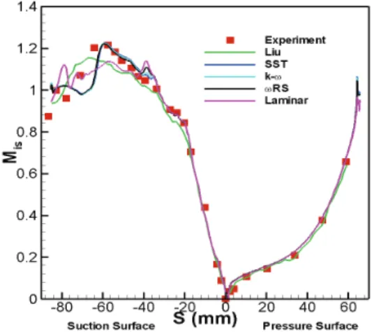
Fig. 9 shows the distribution of the heat transfer coefficients along the blade for present results along with numerical result of Liu[3] and the experimental data[1]

(VKI MUR235). The inlet turbulent intensity (Tu) was 5%

for all turbulent model calculations. In addition, to investigate the effect of the inlet turbulent intensity, Tu = 1% was tested for SST turbulent model. Fig. 9 shows that the effect of changing the inlet turbulence intensity in the current result is negligible. Along the suction side, present results predict early turbulent transition which gives rise to excessively large heat transfer coefficients compared to the experimental data[1]. In fact, most of the RANS based turbulence models do not include built-in transition model and the discrepancy from the experimental data for turbulence sensitive physical quantity like heat transfer coefficient is inevitable without proper addition of turbulent transition model. Liu[3] calculation predicts the transition and heat transfer coefficient better than our three turbulence models do. On the pressure side, our calculations overestimate the heat transfer coefficients on the downstream part, while Liu[3] calculation underestimates it on the whole.

To improve the prediction for the heat transfer coefficient through correct transition,    

[10,11]

correlation-based transition model within the SST model

was tried with several different values of model constant

Fig. 10 Comparison of heat transfer coefficient using transition model

C

[10] in the destruction term. Fig. 10 shows the results of SST turbulence model with model constant C

= 5, 10, and 50, where C

= 50 is the default value[10]. Using C

= 10, the transition was predicted correctly although heat transfer coefficient was somewhat underestimated.

5. C ONCLUSIONS

The numerical simulation of the flow field in a turbine cascade was carried out. The effect of the choice of turbulent model on the flow was investigated. Three turbulence models were tested in addition to laminar case.

The computational results of pressure field around the blade surface for the adiabatic case have shown that all three tested turbulent models produce reasonable agreement with experimental data. However, there was a small deviation between computationally predicated and experimental results on the downstream part of the suction side where stronger shock wave was observed than the experimental data suggest. In the far wake region, all three turbulent models produced correct wake spread rate and ω-Reynolds stress model gave the best match to the experimental data in total pressure loss.

For the isothermal case, computational results of all three tested turbulent models failed to produce correct heat transfer coefficient around the blade surface due to the inability of predicting turbulent transition correctly.

However, computational results were able to be improved

[1] 1990, Arts, T., Lambert de Rouvroit, W., Ruther-ford, A.W., "Aerothermal investigation of a highly loaded transonic linear turbine guide vane," VKI Technical Note 174, Von Karman Institute for Fluid Dynamics, Belgium.

[2] 2008, Liu, Y., "An efficient numerical method for highly loaded transonic cascade flow," J. Eng. Math., Vol.60, pp.115-124.

[3] 2007, Liu, Y., "Aerodynamics and heat transfer predictions in a highly loaded turbine blade," Heat and Fluid Flow, Vol.28, pp.932-937.

[4] 1998, Gehrer, A., and Jericha, H., "External heat transfer pre-dictions in a highly-loaded transonic linear turbine guide vane cascade using an upwind biased Navier-Stokes solver," In Seminar and Workshop on Turboma-chinery Flow Prediction VI.

[5] 1997, Larsson, J., "Turbine blade heat transfer calculations using two-equations turbulence models," J.

of Power and Energy, Vol.211, pp.253-262.

[6] 1989, Barth, T.J., and Jespersen, D.C., "The design and application of upwind schemes on un-structured meshes," AIAA Paper, 89-0366.

[7] 1994, Menter, F.R., "Two-equation eddy-viscosity turbulence models for engineering applications," AIAA J., Vol.32(8), pp.1598-1605.

[8] 2000, Wilcox, D.C., Turbulence Modeling for CFD, DWC Industries, Inc.

[9] 2006, Wilcox, D.C., Turbulence Modeling for CFD, third edition, DCW, Industries, Inc.

[10] 2011, CFX-Solver Theory Guide, Release 13.0, ANSYS Academic Research.

[11] 2009, Langtry, R.B., and Menter, F.R.

"Correlation-based transition modeling for unstructured

parallelized computational fluid dynamics," AIAA. J.,

Vol.47(12), pp.2894-2906.