DOI : 10.5391/JKIIS.2010.20.6.786
접수일자 : 2010년 7월 16일 완료일자 : 2010년 11월 19일
복잡한 환경에서 Grid기반 모폴리지와 방향성 에지 연결을 이용한 차선 검출 기법
Lane Detection in Complex Environment Using Grid-Based Morphology and Directional Edge-link Pairs
림청․한영준․한헌수
Qing Lin, Young-Joon Han and Hern-Soo Hahn 숭실대학교 전자공학과
요 약
본 논문은 복잡한 도로 환경에서 차선을 정확하게 찾는 실시간 차선 검출법을 보인다. 기존의 많은 방법들은 대게 후처리 과정에서 차선 안쪽에 존재하는 잡음을 찾아 차선의 위치를 찾지만, 제안하는 방법은 특징 추출 단계에서 가능한 많은 잡 음을 제거하므로 후처리 과정에서 검색 영역을 최소화한다. grid기반 모폴로지 연산은 우선 관심영역을 능동적으로 생성한 후, 모폴로지의 닫기 연산을 통해 에지 들을 연결한다. 그리고 방향성 에지 연결 기법을 통하여 유효한 방향에지를 찾고 사전에 구해진 영상 내 차선의 높이와 두 차선 간의 폭 관계를 이용하여 두 개의 차선을 군집화한다. 마지막으로 차선의 색상은 YUV색상 공간에서 두 개의 연결된 에지 안쪽을 검사하여 Bayesian확률 모델을 사용하여 추정한다. 제안하는 방법 의 실험 결과는 다수의 불필요한 에지 군집이 존재하는 복잡한 도로 환경에서 효과적으로 도로 에지를 감별하였으며, 제안 하는 알고리즘은 해상도 320×240 영상으로 10ms/frame의 속도에서 약92%의 정확도를 보였다.
키워드 : 차선 검출, Grid기반 모폴리지, 방향성 에지 연결, 라인-템플릿 매칭.
Abstract
This paper presents a real-time lane detection method which can accurately find the lane-mark boundaries in complex road environment. Unlike many existing methods that pay much attention on the post-processing stage to fit lane-mark position among a great deal of outliers, the proposed method aims at removing those outliers as much as possible at feature extraction stage, so that the searching space at post-processing stage can be greatly reduced. To achieve this goal, a grid-based morphology operation is firstly used to generate the regions of interest (ROI) dynamically, in which a directional edge-linking algorithm with directional edge-gap closing is proposed to link edge-pixels into edge-links which lie in the valid directions, these directional edge-links are then grouped into pairs by checking the valid lane-mark width at certain height of the image. Finally, lane-mark colors are checked inside edge-link pairs in the YUV color space, and lane-mark types are estimated employing a Bayesian probability model.
Experimental results show that the proposed method is effective in identifying lane-mark edges among heavy clutter edges in complex road environment, and the whole algorithm can achieve an accuracy rate around 92% at an average speed of 10ms/frame at the image size of 320×240.
Key Words : Lane detection, Grid-based morphology, Directional edge-linking, Line-template matching.
1. Introduction
Lane detection plays an important role in many appli- cations like driving-assistant systems, self-guided ve- hicles, and surveillance systems. Many approaches for lane detection have been proposed and most of them fol- low a similar flow[1]. First, lane-mark feature points are extracted from the road images. Next, a post-processing stage starts to remove outliers and fit the lane-mark feature points to a certain kind of lane model. Many lane
models and fitting algorithms have been proposed.
J.McDonald[2] used Hough transform to fit a linear model. K.Kaliyaperumal[3] proposed Metropolis fitting algorithm to fit a deformable template model. Y.Wang[4]
developed a B-snake lane model with iterative mean square error minimization to fit the parameters. Z.Kim[5]
performed lane detection by using cubic-spline model with RANSAC (RANdom Sample Consensus) algorithm for fitting. Parabolic model is used by J.C. McCall[1] with a statistical and motion based fitting algorithm. In addi- tion, Q.Li[6] proposed a lane detection algorithm which uses adaptive randomized Hough transform to fit the lane boundary without using any pre-defined lane model.
Instead of doing too much careful processing at lane-mark feature extraction stage, most of these meth- ods tend to detect lane-mark features coarsely, while de- pending on the complex fitting algorithm to remove a great deal of outliers for the determination of actual lane-mark positions. On one hand, iterative fitting with coarsely extracted feature points can be more robust in various road conditions for the guarantee of true lane feature existence in coarse feature sets. While on the other hand, large amount of feature points enlarge the searching space of iterative fitting algorithm dramati- cally, resulting in a great increase of the computation cost at the post-processing stage.
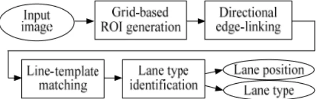
In order to limit the size of the feature space to re- duce the computation cost at the post-processing stage, this paper places a higher value at lane-mark feature extraction stage, that is to identify true lane-mark edges accurately among various clutter edges on the road surface, so as to remove outliers as much as pos- sible at the feature extraction stage. A kind of direc- tional edge-link pair is proposed as a new lane-mark feature, and a directional edge-linking algorithm is de- veloped to extract this kind of feature in a dynamic ROI(Region of Interest) generated by using grid-based morphology operation. At post-processing stage, a sim- ple line-template matching method is used to fit the feature points without heavy iterations. A general flow- chart of the proposed lane detection method is shown in Fig.1. As input of the detection system, lane images are obtained by using an on-board monocular color camera fixed at the front of the vehicle. The output of the de- tection system considers both positions and types of lane-mark.
Fig. 1. Flowchart of the lane detection method.
The rest of this paper is organized as follows: In section 2, dynamic ROI generation by using grid-based morphology is discussed. In section 3, directional edge-linking and grouping algorithm is presented. Lane fitting and type identification is introduced in section 4, including line-template matching, lane-switching de- tection and lane-type estimation. Experimental results are presented in section 5, and final conclusions are made in section 6.
2. Grid-based ROI Generation
Based on intensity variation and color difference be- tween lane-marks and the road surface, a grid-based
morphology method is proposed in this paper to gen- erate a smaller ROI automatically. A diagram of the proposed ROI generation method is shown in Fig.2.
Fig. 2. Flowchart of grid-based ROI generation.
The initial ROI area is set following the general method of excluding the top and bottom areas. Inside this initial region, a grid region, which is composed of 1-pixel wide vertical and horizontal lines, is con- structed, onto which the original image is reduced, as shown in Fig. 3 (1),(2). On this grid region, two sec- ond-difference masks
G
x andG
y are applied to R and B channels of RGB image in the horizontal and vertical directions separately. A pixel is retained only if the mean value of the separable convolution in R and B channel reaches a predefined threshold. The horizontal and vertical gradients∇ H
,∇ V
are defined in (1), whereI
r represents R channel andI
b indicates B channel.[1 0 1]
[1 0 1]
x
T y
G G
= −
= −
2 2 (| * | | * |) / (| * | | * |) /
r x b x
r y b y
H V
I G I G
I G I G
∇ =
∇ =
+
+ (1)
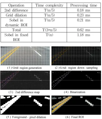
Since lane-marks usually have specific colors like yel- low, blue and white, and these color pixels usually have dominant values in the R and B channel. By applying second-difference operators to R and B channel sepa- rately, and making the final pixel decision based on the separable convolution results in these two channels, grid-edge components that contain lane-mark pixels can be extracted efficiently, as shown in Fig.3 (3)(4). Based on the extracted grid-edge components, grid-cells are filled by using a dilation operation to the foreground pix- els with a 10×10 square element, and the filled dilation region is the final ROI which contains lane-mark pixels.
The final ROI results are shown in Fig.3 (5) (6).
In addition, since the separable convolutions are con- ducted on a grid-sampled image, the pixels involved in convolution calculations are much less than that in the original image. Therefore, this grid-based convolution and dilation operation can be executed very quickly.
Table 1 shows the speed comparison between using dynamic ROI and fixed ROI. In Table 1, for simplifying, time complexity is described using the number of pixels that require assignment operations or arithmetic calculations. Without using dynamic ROI, the Sobel op- erator has to be applied to almost every pixel in the fixed ROI. While grid down-sampling operation can re- duce the number of pixels to 1/5 of the original amount, so that the following operations can work at the time complexity of T(n/5).
Operation Time complexity Processing time 2nd difference T(n/5) 0.18 ms
Grid dilation T(n/5) 0.23 ms Sobel in
dynamic ROI
T(n/5) 0.21 ms
Total T(3*n/5) 0.62 ms
Sobel in fixed ROI
T(n) 1.18 ms
Table 1. Processing-time comparison of using dynamic ROI and fixed ROI.
Fig. 3. ROI generation using grid-based dilation.
3. Directional Edge-link Pairs
Many lane-mark feature extraction methods have been proposed. Some use lane-mark textures and learn- ing-based method to train a lane-mark classi- fier[7].Other methods mostly depend on edges[8][9].
Edge-based methods can work well with either solid or dashed lane-marks, and can be largely invariant to illu- mination changes. However, many edge-based techni- ques can often fail in situations where many extraneous lines exist. The proposed edge-based feature extraction method is able to identify true lane-mark edges even in these difficult situations, which makes the lane de- tection algorithm more adaptive to complex environments. Three steps, including edge detection, di- rectional edge-linking with edge-gap closing, and edge-link pair grouping are used to obtain possible lane-mark edges as accurate as possible.
3.1 Edge detection
In the edge detection step, a Sobel operator is firstly used to find edge-pixels inside the ROI. For the pixel set
I '
inside ROI, a Sobel operator is applied to com- pute gradient amplitudes| ( * ') | ∇ G I
as defined in (2).1 0 1 2 0 2 1 0 1
Gx
⎡ − ⎤
⎢ ⎥
=⎢ − ⎥
⎢ − ⎥
⎣ ⎦
1 2 1 0 0 0 1 2 1
⎡ ⎤
⎢ ⎥
= ⎢ ⎥
⎢− − −⎥
⎣ ⎦
Gy
∇f(x,y
)=⎡ ⎣
( '* )I Gx
2+( '*I Gy
)2⎤ ⎦
1 2/ (2)Local gradient orientations can also be found by checking the sign of
I G ' ∗
x andI G ' ∗
y. Gradient ori- entation features for left and right lane boundaries can be used to remove invalid edge-pixels for left and right lane-mark. In addition, they can also be used to identify inner and outer boundaries of lane-marks in the edge-link pair grouping stage.3.2 Directional edge-linking
After edge map is obtained, a directional edge-linking algorithm is used to find candidate edge-pixels which lie on lane-mark boundaries. Edge-linking is a very ef- fective method to find object boundaries in certain geometries. In this paper, the general edge-linking al- gorithm is extended to identify lane-mark edge geome- try in a noisy edge map.
Edge-link is defined as a vector which contains 5 parameters <
ID P
, head,P L
tail, , ,α . ‘ID’ is the label of this >edge-link, ‘
P
head’ and ‘P
tail’ is the starting point and end point, ‘L’ is the length, and ‘α
’ is the direction of this edge-link. The direction of edge-link is described by unit-direction and main-direction. The unit-direction is defined according to the orientations of one pixel’s 8 neighborhoods, as shown in Fig.4. Based on the defi- nition of unit-direction, the main-direction of edge-link is defined as the mean value of all unit- directions be- tween every two neighboring pixels:α = ∑ U L
i/( − 1)
, whereU
i∑
represents the sum of all unit directions. An exam- ple of main-direction calculation is illustrated in Fig.4.Directional edge-linking algorithm is developed based on an 8-neighborhood edge-pixel tracing algorithm. The directional edge-linking algorithm is composed of two steps: starting point scan and edge-pixel tracing.
45 90 45 90 4 67 5 (
D+
D+
D+
D) / = .
D45 D 90 D 135 D 180 D
225
D270
D315
D0
DFig. 4. The definition of edge-link direction.
During the edge-pixel tracing process, basic and ef- fective unit-directions are introduced to guide the tracing. The definition of basic and unit directions are shown in Fig.4.
The edge-point tracing process continues until one of the following two conditions are met: (1) No more con- nected edge-pixels can be found. (2) The unit-direction of the next neighboring edge-pixel falls out of effective direction range. In either case, the current edge-link will terminate, and a new edge-link will be initialized in
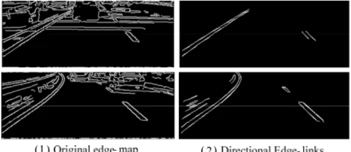
the starting point scan process. Finally, when no more unlabeled starting points can be found, the whole edge-linking process will terminate, then the main-di- rection and length of each edge-link are checked. The main-direction of edge-link should lie between 30° to 150°. The length of edge-link should be larger than a threshold value as well. All edge-links that violate this rule are not likely to be lane-mark edges and are therefore discarded. Some results of proposed edge-linking algorithm are shown in Fig.5.
Comparing with the edge-linking algorithm based on chain-code as the one used in [10], the proposed direc- tional edge-linking algorithm introduced unit-direction and main-direction to describe edge-link path in a much finer way, which is able to track many edge-link paths within the valid lane-mark direction range that chain-code based edge-linking algorithm can not capture.
Fig. 5. Directional edge-linking result.
3.3 Directional edge-gap closing
The above directional edge-pixel linking algorithm works well on edge images obtained from an original resolution image with little noise. However, due to noise and pixel loss caused by down-sampling operation, some dashed lane-mark edges which appear in the far field of camera-sight will be broke up into many small disconnected segments. Since the lengths of these small links are usually under the edge-link length threshold, they can be easily filtered out as noise edge-links, which cause the loss of real lane-mark edges. This is illustrated in Fig.6.
Fig. 6. Directional edge-gap closing result.
To deal with this problem, a directional edge-gap closing algorithm is added to produce more complete edge-links. After edge-links with valid orientations are obtained, the directional edge-gap closing step begins.
In this step, edge-links are extended by adding new edge-pixels along the edge-link orientation to fill the possible gaps which split a complete edge-link. The maximum number of added points is determined by a user-defined value. Generally, 5 pixels are enough to fill the gaps between split edge-links.
New edge-points are selected from the neighboring points of the starting point and end point of one edge-link along the edge-link orientations. As Fig.7 il- lustrates, on a gradient image, for a given edge-link, three points
G
1,G
2, andG
3, which lie in the effective di- rection around tail point are considered as candidates for new edge-points. If the gradient values ofG
1,G
2 andG
3 are larger than a gap-closing threshold, then for each of these three candidate points, a gap-closing score is calculated as:M
i=G
i+max(G G G
ni1, ni2, ni3), whereG
i indicates the gradient value at the ith candidate points, whileG G G
ni1, ni2, ni3 refer to the gradient values at the three neighboring points around ith candidate points.The sum of the candidate point’s gradient and the max- imum gradient of this point’s three neighbors is calcu- lated as a gap-closing score
M
i. The point with the maximum gap-closing score is finally selected as the new edge-point to be added to the edge-link. This edge-link extension process will continue until one of the three following conditions is satisfied:(1) The point in another edge-link is detected in the neighborhood of newly added edge-points. This means two edge-links meet each other, so that they are merged into one complete edge-link.
(2) The maximum number of new points is reached.
(3) There are no more points with gradient value larger than the minimum gap-closing threshold can be found.
G
1G
2G
3 11
G
n 2 1G
n 31
G
n 12
G
n 22
G
n 32
G
n1 3
G
nG
n23 3 3G
nFig. 7. Directional edge-gap closing algorithm.
After directional edge-gap closing, those disconnected small segments which belong to one lane-mark can be linked together as one edge-link. Then edge-link length is checked to discard those small edge-links with lengths below threshold. The effect of this directional edge-linking algorithm is shown in Fig.6.
3.4 Edge-link pair grouping
After candidate edge-links are obtained, edge-link pair grouping is carried out based on the distance be- tween adjacent edge-links. If the distance satisfies the width of a lane-mark at certain height of the image, then the region enclosed by this pair of edge-links will be regarded as candidate lane-mark regions.
In scanning, edge points with opposite gradient val- ues along horizontal direction are selected as candidate matching points for lane boundaries. When a pair of potential matching points P
1
and P2
are found, the hori- zontal distance between P1
and P2
is calculated and compared with the corresponding width value in the look-up table. If satisfied, then the point counters of the edge-links which contain P1
and P2
will increase by 1.In every row of the edge-link image, the matching points P
1
and P2
are searched and recorded in the point counters of their corresponding edge-links, a likelihood score is estimated ass
k= ∑ C
j/ ∑ E
i, where∑ C
j is the total number of edge-points recorded in the point coun- ter of edge-link k, and∑ E
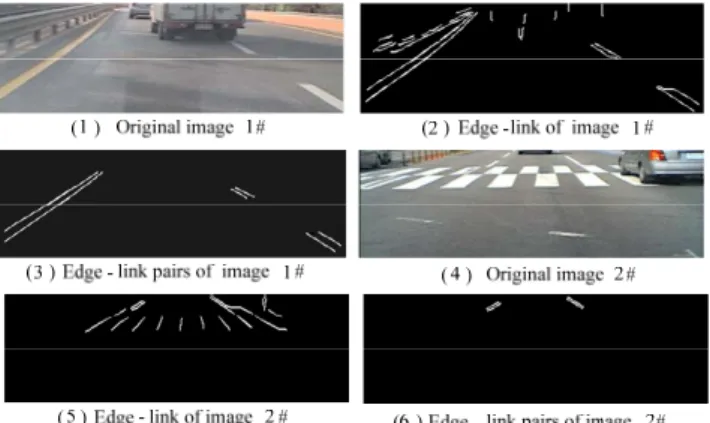
i is the total number of edge-points which edge-link k contains. Finally, ad- jacent candidate edge-links with opposite gradient di- rections are grouped into pairs. And the region enclosed by edge-link pairs is regarded as candidate lane-mark regions.By scanning edge-links with lane-mark width, some edge-links caused by road signs or guardrails which have similar orientations as lane-mark edges, can be removed. Some results are shown in Fig.8.
Fig. 8. Directional edge-link pair grouping result.
4. Lane Fitting and Type Identification
After directional edge-linking and grouping, edge-link pairs that are most likely to be lane-mark boundaries can finally be decided. A simple line-template matching algo- rithm is used here to fit the lane position very efficiently.
4.1 Line-template matching
In the coordinate system given in Fig.9, the line
equation given in (3) is used for generating the line-templates. The line-template is determined by two points (x1, y1) and (x2, y2), which are located on this line. In Fig.9, line R is set as the range to which line models are fitted.
1 2 1
1
2 1
( x x y )( y )
y y
x x
− −
= +
−
(3)Fig. 9. Line-template matching.
The line-template based fitting algorithm is com- posed of two parts. The first part is searching range estimation. By extending every edge-link using a straight line, and calculating its intersection points on line R and the image boundaries, a cluster of inter- section points on line R and the image boundaries can be obtained, and the distribution range of these inter- section points can be estimated. As shown in Fig.9 (1), the range enclosed by X1 and X2 on line R, and the range enclosed by Y1 and Y2 set the searching range for right lane.
In the line-template generation and matching step, as is shown in Fig.9(2), for one point on line R starting from X1, a set of line-templates is generated based on equation (3) by simply connecting point on line R with every point on the right image boundary from Y1 to Y2. And on each line-template, the number of edge points which overlap with this line-template is calcu- lated as the matching score of this line-template. After one set of line-templates is generated, the point on line R will move forward to the next point, and another set of line-templates is generated. Finally, when it moves to X2, the total number of line-template that are gen- erated is (X2-X1)×(Y2-Y1). Among all those line-tem- plates, the one with the highest matching score is se- lected as the best matching template.
4.2 Lane switching detection
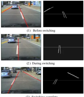
The way to identify lane switching is to check the position of two end-points (x1, y1) and (x2, y2) of the fitted line. If two end-points of the right fitting-line is moving to the left of the middle-point of image, then it is regarded that the vehicle is switching to the right lane. When lane switching happens, the direction of lane-mark which the vehicle is crossing will be around 90°, directional edge-linking algorithm can still work effectively in this case to get the boundaries of switch-
Frames Correct Detection
False Detection
Miss Detection
3000 2770
(92.3%)
145 (4.82%)
85 (2.88%) ing lane-mark. An example of the right-lane switching
process is shown in Fig.10, in which the left image shows lane fitting result, and the right image shows the extracted directional edge-link pairs.
(1) Before switching
(2 ) During switching
(3) Switching complete
Fig. 10. Example of right-lane switching.
4.3 Lane type identification
Lane types can be identified by specific color and continuity. In Korea, there are generally three kinds of lane-mark colors: white, yellow and blue. These three colors are much easier to identify in the YUV color space. Therefore, color identification is done in the YUV color space. By using adaptive thresholds calculated from local histogram, yellow, blue, and white dominant regions can be extracted from the U, V and Y channels.
Scanning candidate lane-mark regions enclosed by edge-link pairs on yellow regions first, and then calcu- lating
R
yi/ R
i,R
yi indicates the number of yellow pixels inside the candidate lane-mark region, whileR
i means the total number of pixels inside candidate lane-mark region. If this ratio is larger than a threshold value, it is assumed that this region contains yellow lane-marks.Blue and white colors are checked in the same manner.
In terms of the continuity of lane-mark, it can be classified as solid lane-marks and dashed lane-marks.
In order to identify the continuity of lane-mark, a Bayesian probability model is employed. Given the best matching line-template L, two posterior probability functions (4) and (5) are involved to estimate the type of lane-mark, where
P( | L Solid )
andP( | L Dash )
are the likelihood of solid and dashed lane-marks, whileP( Solid )
andP( Dash )
are the corresponding prior probabilities.P( Solid | ) L = P( Solid )P( | Solid) L
(4)P( Dash | ) L = P( Dash )P( | L Dash )
(5)Therefore, the given best matching line L can be classified as solid or dashed by using the following Bayes decision rule:
P( | P( | )
P( | P( | )
) )
solid solid dash dash solid dash
∈ ≥
<
⎧ ⎨
⎩
L L
L L L
(6)The prior probability
P( Solid )
andP( Dash )
can be esti- mated using some prior knowledge. For example, by using lane-mark colors appear on a specific type of road. This is based on the prior knowledge that, in Korea, most yellow and blue lane-marks that appear on city roads or highways are solid lane-marks, while white lane-marks are usually dashed lane-marks on the city road. The likelihood is calculated based on the ratio between the number of overlapped edge-pixels on the fitted line and the real length of the fitted line, as is shown in (7),P( | )
t/
jt j
Solid = ∑ ∑ E L
L
(7)5. Experimental Results
The proposed lane detection algorithm has been im- plemented in visual c++ 6.0. For video clips with 320×240 image size, the processing time is around 10ms per frame on an Intel Core2 1.86GHZ processor.
To evaluate the performance of the proposed lane de- tection algorithm, the detection results on a road vid- eo-clip with very complex environment are presented here. The video clip used for testing is very challenging since it contains different lane types, all kinds of lane variation situations (emerging/terminating/merging/
switching/intersecting), complex road surfaces (clutter markings, shadows), and significant obstacles (vehicles running on the road).
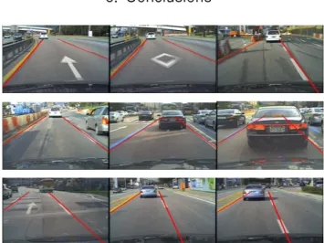
The test results on this video clip are shown in Table 2. 3000 frames from this video clip are used for testing. Here “Correct Detection” means all lane param- eters including number of lanes, lane position, color, and continuity are correctly detected. If one parameter is not correctly detected, then the result is reported in “False Detection”. In addition, in cases where non-lane objects are detected as lane are also included in “False Detection”. On the other hand, if existing lanes are not detected, then these cases are reported in “Miss-de- tection”. Fig.11 lists some examples of the detection results.
Table.2 Test results on video clip
6. Conclusions
Fig. 11. Examples of detection results.
In this paper, a lane detection method based on grid-based morphology and directional edge-link pairs is presented. Compared with other lane-detection meth- ods, the proposed algorithm pays much attention at the feature extraction stage to achieve a much higher proc- essing speed. Since most of the noise and outliers can be removed at feature extraction stage, this helps to limit the searching space for the fitting algorithm, so that the computation cost for line-template matching can be greatly reduced. Meanwhile, in the proposed al- gorithm, there are no special requirements for any cam- era parameters or background models. This makes the algorithm more adaptive to various road environments.
References
[1] J. C. McCall and M. M. Trivedi, “Video-based lane estimation and tracking for driver assistance: sur- vey, system, and evaluation,” IEEE Trans. Intell.
Transp. Syst., vol. 7, no. 1, pp.20-37, 2006.
[2] J. McDonald, “Detecting and tracking road markings using the hough transform,” Proc. of
the Irish Machine Vis. and Image Processing Conf., pp. 1-9, 2001.
[3] K. Kaliyaperumal, S. Lakshmanan, K. Kluge,
“An algorithm for detecting roads and obstacles in radar images,” IEEE Trans. Veh. Tech., vol.
50, no. 1, pp.170-182,2001.
[4] Y. Wang, E. K. Teoh, D. Shen, “Lane detection and tracking using B-snake,”
Image Vis.
Comput., vol. 22, no. 4, pp.269-280, 2004.
[5] Z. Kim, “Robust lane detection and tracking in challenging scenarios,” IEEE Trans. on Intell.
Transp. Syst., vol. 8, no. 1, pp. 16-26, 2008.
[6] Q. Li, N. Zheng, and H. Cheng, “Springrobot: A prototype autonomous vehicle and its algorithms for lane detection,” IEEE Trans. Intell. Transp.
Syst., vol. 5, no. 4, pp. 300-308, 2004.
[7] J. W. Park, K. Y. Jhang, J. W. Lee, “Detection of lane curve direction by using image process- ing based on neural network and feature ex- traction,” Journal of imag. sci. and tech., vol. 45, no. 1, pp.69-75, 2001.
[8] J. Park , J. Lee and K. Jhang, “A lane-curve detection based on an LCF,” Pattern Recognit.
Lett, vol. 24, no. 14, pp.2301-2313, 2003.
[9] M. Sotelo, F. Rodriguez, L. Magdalena,
“VIRTUOUS : vision-based road transportation for unmanned operation on urban-like scenarios,”
IEEE Trans. Intell. Transp. Syst, vol. 5, no. 2,
pp.69-83, 2004.[10] J. Yu, Y. Han, H. Hahn, “A scheme of extract- ing forward vehicle area using the acquired lane and road area information,” Journal of Korean
Institute of Intell. Syst, vol. 18, no. 6, pp:
797-807, 2008.
저 자 소 개
림 청 (Qing Lin)
2003년 : 산동과학기술대 컴퓨터학과 졸업.
2003년~2009년 : 산동과학기술대 강사 2009년~현재 : 숭실대학교 전자공학과
석사과정
관심분야 : 영상처리, 물건검출, 임베디드 시스템 Phone : 02-821-2050
E-mail : [email protected]
한영준 (Young-Joon Han)
제 14권 7호(2004년 12월호) 참조
한헌수 (Hern-Soo Hahn)
제 13권 4호(2003년 8월호) 참조