확률모델을 이용한 산림전용지역의 스크리닝방법 개발
이정수1※
Development of a Screening Method for
Deforestation Area Prediction using Probability Model
Jung- Soo LEE1※
ABSTRACT
This paper discusses the prediction of deforestation areas using probability models from forest census database, Geographic information system (GIS) database and the land cover database. The land cover data was analyzed using remotely-sensed (RS) data of the Landsat TM data from 1989 to 2001. Over the analysis period of 12 years, the deforestation area was about 40ha. Most of the deforestation areas were attributable to road construction and residential development activities. About 80% of the deforestation areas for residential development were found within 100m of the road network. More than 20% of the deforestation areas for forest road construction were within 100m of the road network. Geographic factors and vegetation change detection (VCD) factors were used in probability models to construct deforestation occurrence map. We examined the size effect of area partition as training area and validation area for the probability models. The Bayes model provided a better deforestation prediction rate than that of the regression model.
KEYWORDS: Deforestation, Probabilistic Prediction, Bayes Model, Regression Model, Geographic Information System, Remote Sensing
요 약
본 연구에서는 행정정보, GIS, RS정보, 확률모델을 이용하여 교토의정서에서 정의하는 산림전용 지역의 추출가능성에 대하여 검토하였다. 1989년의 정사사진과 2001년의 IKONOS화상을 이용한 산림전용지역의 특성을 보면, 1989년부터 2001년까지의 산림전용지역은 약 40ha로 나타났다. 산림 전용지역의 종류를 살펴보면, 도로(임도) 개설 및 주택지 개발을 위한 산림전용이 대부분을 차지하 였고, 택지전용지의 80%는 기존의 도로로부터 100m이내에 분포하였으며, 신설된 도로 또한 20%
이상이 기존의 도로로부터 100m이내에 분포하였다. 산림전용지역의 추출모델 구축을 위하여 지형
2008년 5월 6일 접수 Received on May 6, 2008 / 2008년 5월 30일 수정 Revised on May 30, 2008 / 2008년 6월 9일 심사완료 Accepted on June 9, 2008
1 강원대학교 산림환경과학대학 산림경영조경학부 Division of Forest management and Landscape Architecture, College of Forest Environmental Sciences, Kangwon National University
※ 연락저자 E-mail : [email protected]
인자와 위성영상인자를 이용하였으며, 확률 개념을 도입한 산림전용지 발생 확률 지도를 작성하였 다. 구축한 산지전용지 발생 모델의 유효성을 검증하기 위하여, 대상지역을 시스템적으로 구분하 여, 추출 정도를 비교·검토하였다. 베이즈 모델과 Regression모델을 비교한 결과, 베이즈모델이 Regression모델보다 높은 추출확률을 나타냈다. 모델의 적합성을 평가하기위해서 대상지역을 2지 역으로 구분하여 한쪽의 정보만을 가지고 발생확률지도를 작성하고, 나머지 지역에 대하여 발생확 률을 검토한 결과에서도 베이즈모델이 높은 추출확률을 나타냈다.
주요어 : 산림전용, 확률예측, 베이즈모델, 회귀모델, 지리정보시스템, 원격탐사
INTRODUCTION
Article 3.3 of the Kyoto Protocol prescribes that three types of activities- afforestation, reforestation and deforestation are to be reported when accounting for forest sinks to compensate for greenhouses gases (GHG). Afforestation(A) is defined as
"direct human-induced conversion of land that has not been forested for a period of at least 50years to forested land," reforestation(R) as "the direct human-induced conversion of non-forestedland to forested land," and deforestation (D) as "the direct human- induced conversion of forested land to.
Kyoto protocol designates deforestation as required reporting item.
Monitoring of forest change area should be possible assessed by remote sensing using aerial photos and satellite images.
Although monitoring forest changes with satellite data includes land cover changes, articles 3.3 and 3.4 of the Kyoto Protocol require the monitoring of both land-use changes and land-cover changes. But because satellite remote sensing (RS) provides only land-cover spectral information, RS by itself is not sufficient for identifying LULUCF (Land use, Land-use change and forestry). Recently, to overcome the detection limitations of RS, RS and GIS
techniques were recently combined with administrative information to improve forest change detection (Kodani, 2003; Hori et al., 2002).
On the other hand, quantitative methods have been applied to various disciplines such as Land-use and Land-cover classification (Elmore et al., 2000), forest structure monitoring (Franklin, 1986) and landslide hazard prediction (Carrera et al., 1991;Chung et al., 1995;Chung and Fabbri., 2003).
Geometric probability based models (Fabbri and Chung,1996;Chung and Fabbri, 1999), statistical pattern integration and spatial reasoning will be useful to deforestation monitoring. Therefore, the development of methods that can be used to estimate deforestation areas in changing forest regions, as well as accompanying quantitative methods, will be useful in future studies.
In this study, we proposed a new approach by linking Geographic Information system(GIS), RS and probability models that can be used to identify deforestation area accurately.
METHODS
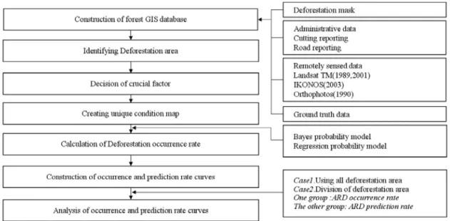
Figure 1 shows the methodology proposed in this study. The deforestation masks were obtained from satellite images and ground truth. GIS databases related to the deforestation areas were constructed from map sources.
Figure 1. Method of prediction model
Factors for building the prediction model were identified from the geographic attributes of deforestation. These attributes were slope, distance from road network, and distance from forest and non-forest (F/NF) boundaries. In addition, vegetation change detection (VCD) based on Landsat TM band3 was also used as critical factors. The occurrence and prediction rates of deforestation were calculated for each factor.
Two joint conditional probability models (Bayes and regression estimation) were applied to every pixel of the deforestation areas and then used to construct a probability model.
The deforestation areas were divided into two sub areas in the model. One area was used to construct the deforestation occurrence rate model, the other was used to construct the deforestation prediction model.
To obtain the deforestation prediction map, estimated probabilities of occurrence
were sorted in descending order. The ordered pixel values were then classified according to the rates of deforestation in the sub area. The occurrence rate curve (ORC) and prediction rate curve (PRC) were compared in terms of the proportion of corresponding pixels.
Description of study area
Higashi-Shirakawa area was selected as a test site for this study. Based on the criteria of agricultural zoning, the study area is classified as hilly and mountainous area.
Higashi-Shirakawa area is located in the southeastern part of Gifu Prefecture, Japan.
and includes part of the wide valley of the Shirakawa River. It covers approximately 15 by 15km and 8,711ha.(Longitude 137°15'24"
to 137°24'35", Latitude 35°41'46" to 35°35'51"). More than 90% (8,013ha) of the study area is covered with forest. However, the forest was dominated by plantation
forest (5,759ha). The test site receives mean annual precipitation of 2,258mm, The mean temperature ranges from -15°C to 34°C, with a mean of 12.9°C.
Data acquisition and processing
TNTmips version 6.9 of Microimages was used for data processing and analysis. The remotely-sensed data sets used were medium-resolution Landsat TM images (1989/06/01, 2001/05/27), high-resolution satellite IKONOS image (PAN, 2003/07/26) and Digital-Orthophoto(1990/05). We performed geometric and radiometric corrections for satellite data (Smith et al., 1980).
Topographic effect due to surface slope angle and aspect variations was corrected for the Landsat TM. Instead of lambertian approach, the non-lambertian empirical photometric function outlined by Smith et al.(1980), based on a principle developed by Minnaert, was used to correct topographic effects. Relative normalization was applied to Landsat TM data for correcting the radiance difference in the multi-temporal data. Spatial forest management information including compartments, sub-compartments (1:5,000), and road networks (1:5,000), was digitized as a GIS database.
The land cover change mask was produced using high-resolution remotely sensed images (orthophotos and IKONOS image) and groundtruth data. The land cover change mask defines the ARD mask, which consists of five categories i.e.permanent clearcut, forest road, slope-facing, tea plantation establishment, agricultural road and afforestation area.
Joint Conditional Probability Model
This study used the joint conditional model, proposed by Chung and Fabbri (1999), which can identify correlations between the positions of past deforestation areas and spatial data. Two joint conditional probability models (Bayes and regression estimation) were applied to every pixel of the deforestation areas and then used to construct a probability model.
Suppose that denoting a pixel that will be affected by a future occurrence of deforestation. Future deforestation area at each pixel can be expressed as a joint conditional probability:
⋯ ⋯
∩
(1)
And, past deforestation area at each pixel
is expressed by the following joint conditional probability:
⋯ ⋯
∩
(2)
Where S represents the areas affected by the past deforestation areas within A.
The deforestation area layer in addition to the four attribute layers in the study area, were used in the probability model (Figure 2b). In the data set, 81 variables (3×3×3×3 =
81) were obtained from four data layers including the distribution of past deforestation areas. therefore, each pixel in a thematic classification map has a set of values such as (1,1,1,1), (1,1,1,2),....,(3,3,3,2), (3,3,3,3), depending on the combination of three categories of four thematic maps. All pixels where the observed values of the m layers that are identical were termed
"unique condition sub-areas". The study area can be subdivided into a small number of unique condition sub-areas. ∩
represents the presence of deforestation area in pixel of unique condition based on the combination of the attribute layers (
).
Using the Bayes theory(Bayes, 1763), the joint conditional probability is shown as below:
⋯
⋯
⋯
⋯ ⋯
⋯
⋯
(3)
: The size of S
:The size of ∩
Bayes theory was applied to the joint conditional probability model, which considered prior probability and posterior probability conditions simultaneously. In addition, A multivariate linear regression model for the conditional joint probability in Equation 4 for a pixel p can be postulated by
⋯
⋯
(4)
Categorization of crucial factors and for deforestation prediction
1) Geospatial factors
Selection of crucial factors is an important aspect for building the deforestation probability model. By the basic proposition of probability model, categorization of selected factors is necessary for building a model.
Two accessibility factors, namely
"distance from road to deforestation" and
"distance from forest and non-forest (F/NF) boundary to deforestation" were selected as the crucial factors of the model. Forest area, non-forest area and road were derived from compartment data. The two accessibility factors, distance from road to deforestation and distance from forest and non-forest (F/NF) boundary to deforestation, were derived from compartment data and a DEM(Digital elevation model).
The two accessibility factors were categorized into multiple classes of 150m interval. The slope factor was categorized based on reports of studies on quantification and evaluation of forest functions by Forestry Agency (Forestry Agency, 1998).
Table 1 shows the categories of the three geospatial factors.
2) Vegetation change detection (VCD) factor Image differencing technique is an effective analytical method for detecting
deforestation using satellite data especially for forest clearing where change brightness value is very significant. Image differencing may be applied to a single band or to multiple bands. It is a simple and straightforward approach where changes in a pixel at line i and column j of band k (bvCijk) is computed as below:
bvCijk=bvijk(d2)- bvijk(d1) bv : brightness value
d2 and d1 : date 2 and data 1,respectively Differenced image resulted from the subtraction of two multitemporal images represents the change between the two dates. The change pixels can be expected to lie in the tails of the distributions of the differenced image, whereas the unchanged pixels should be grouped about the mean.
In this study, image differencing techniques was applied on red (R) band i.e.
band 3. Red (R) and near infrared (NIR) bands of remote sensing data are important to vegetation studies. R band comprises absorption wave lengths of chlorophyll of green vegetation (Tucker and Maxwell, 1976).
The resulted band3 of VCD images were also categorized to three classes by thresholding based on statistical measures (mean and standard deviation (std)).
Standard deviation from the mean is often employed and has been found suitable to determine change and no change area (Eastman and Mckendry, 1991). defined by VCDijk value lower than 1×std + mean is vegetation decrease class, otherwise vegetation increase class (VCDijk value >
1×std + mean). No change class is defined by VCDijk values that fall within the standard deviation range.
Construction of occurrence rate curve
Deforestation occurrence rate curve is based on the comparison between deforestation areas and the deforestation occurrence probability of the study area used in the two models. The deforestation occurrence probability was calculated and sorted in descending order. The number of pixels of the probability value and the corresponding deforestation areas were counted for the whole study area. The deforestation occurrence rate was calculated by dividing the number of deforestation pixels of the probability value with the total number of pixels of that probability value.
Spatial partition and model performance
In prediction modeling, one of the most important components is to validate the predicted results. Without validation, the prediction model is less valuable and scientifically unsound (Chung and Fabbri, 2003). Ideally, a prediction model should be validated by comparing the predicted result and the future deforestation area. Alternatively, the study area can be partitioned to construct and validate the model. We divided the study area into two sub-areas, A and B.
Sub-area A was for constructing the model, while sub-area B was for validation of the predictedresults(Figure 3).
RESULTS AND DISCUSSION
1. The Characteristics of deforestation area Exploratory analysis on the GIS, RS and
(a) (b)
Figure 2. Crucial factor of categorization
a. Half portion partition b. Grid-type into two groups
: A : B
Figure 3. Two types of spatial partition
Category
Factor 1 2 3
Slope -15 16-30 31-
Distance from road (m) -150 151-300 301-
Distance from F/NF boundary (m) -150 151-300 301-
VCDband3 -2 3-17 18-
Table 1. GIS data layers for prediction model
forest census data revealed that distance from road network is the most crucial deforestation factor where 54% of deforestation was distributed from the road within 100m. This is followed by the distance from the forest and non-forest boundary where 39% of deforestation was found within 300m. Most of the deforestation areas were attributed to road construction activities, which account for about 80% of the deforestation areas. The forest was cleared to make way for construction of forest and agricultural roads.
Deforestation due to slope cutting for road construction has also contributed to deforestation. Forest clearing for residential development has accounted for about 10% of the deforestation areas. About one-third of the deforestation areas for residential development were found within 100m of the forest and non-forest boundary.
2. Comparison of the joint probability models
1) Harf portion partition and model performance
We first examined the deforestation occurrence rates of the two probability models (Bayes and regression).We divided the study area into 2 sub-areas, namely sub-area A and B. The sub-area A was for constructing the model whereas the sub-area B was for validating the predicted results(Figure 3a).
The deforestation areas induced by the ARD mask were 390 pixels and 95 pixels for the sub-area A and the rest in sub-area B. While sub-area A was used for
occurrence estimation. The validated prediction image was constructed in sub-area B using the model built from sub-area A.
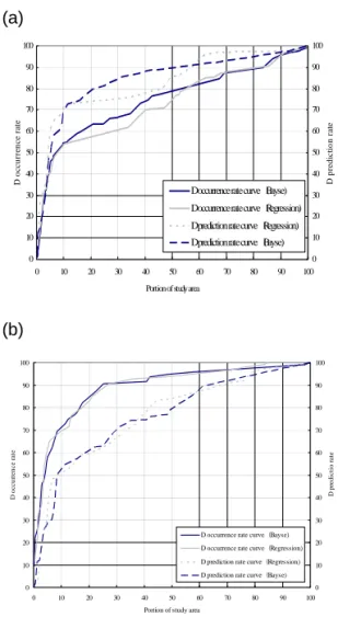
Using the Bayes and regression models, the deforestation occurrence and prediction rates were calculated. For instance, when 20% of the study area is considered, the occurrence rate is 63% (Figure 4a). Obviously, the occurrence and prediction rates increase with the increase in the portion of the study area considered. Thus, an ideal model should be the one achieving the highest accuracy for the smallest assigned portion of the study area. Figure 4 shows deforestation occurrence rate curve (D-ORC) and deforestation prediction rate curve(D-PRC) with the half portion partition. In the case of the Bayes model, the agreement between the D-ORC and the D-PRC was very high for the top 5% of the study area (Figure 4a). When the sub-areas A and B were reversed, disparity of the D-ORC and D-PRC of the Bayes model was observed but relatively acceptable compared to the regression model (Figure 4b).
At this stage, it was premature to draw any conclusion on the performance of the models but the partition assignment seemed to produce a more profound influence on the regression model than the Bayes model. The half-portion partition was a very large spatial unit that about 80% of the deforestation areas were found in one half portion partition. When the sub-areas were reversed, the deforestation areas were too small for training the models and thus influenced the consistency of the results. A different partitioning strategy was therefore
(a)
0 10 20 30 40 50 60 70 80 90 100
0 10 20 30 40 50 60 70 80 90 100
Portion of study area
D occurrence rate
0 10 20 30 40 50 60 70 80 90 100
D prediction rate
D occurrence rate curve(Bayse) D occurrence rate curve(Regression) D prediction rate curve(Regression) D prediction rate curve(Bayse)
(b)
0 10 20 30 40 50 60 70 80 90 100
0 10 20 30 40 50 60 70 80 90 100
Portion of study area
D occurrence rate
0 10 20 30 40 50 60 70 80 90 100
D predictio rate
D occurrence rate curve(Bayse) D occurrence rate curve(Regression) D prediction rate curve(Regression) D prediction rate curve(Bayse)
Figure 4. D-ORC and D-PRC using two sub-areas (a)Sub-area A was used as training area and sub-area B was used as validation area (b) Training area and validation area were reversed from(a)
necessary to improve the performance of the models.
2) Systematic grid partition and model performance
We further examined the effect of partition assignment by further partitioning
the study area into smaller grids of 316m by 316m. The grids were systematically selected for modeling and validation. As such, the deforestation areas were more or less equally divided for modeling and validation. There were 246 pixels and 239 pixels of the deforestation areas in grid groups A and B. Similar to the previous section, the grid groups A and B were used as training area and validation area at first.
Then, they were reversed for comparison (Figure 3b).
Figure.5a and b show the influence of the systematic grid partition on the Bayes and regression models. Compared to the half partition, the difference between the occurrence and prediction rates was substantially small in both Bayes and regression models (Figure 5a). Reversing the grid groups has not resulted significant difference in the occurrence and prediction rates (Figure 5b). Summing the difference between the occurrence and prediction rates can also represent the consistency. The sum of difference of the Bayes model was significantly lower than that of the regression model, in both assignments of grid groups. While difference of occurrence and prediction rates from Bayes model was below 9%, difference of regression model was about 13%.
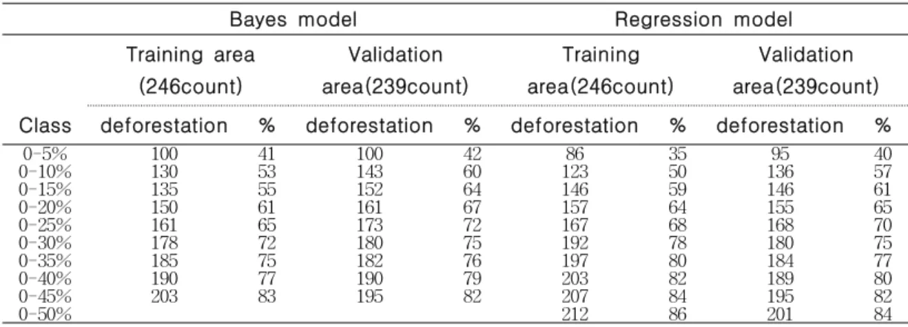
Tables 2a and b show the occurrence and prediction rates of the Bayes and regression models with the systematic grid partition.
Table 2a shows the occurrence rate and prediction rate calculated using grid group A and B, respectively. Table 2b shows the results when the use of the groups was reversed. For the top 10% class, the Bayes
0 10 20 30 40 50 60 70 80 90 100
0 10 20 30 40 50 60 70 80 90 100
Portion of study area
D occurrence rate
0 10 20 30 40 50 60 70 80 90 100
D prediction rate
D occurrence rate curve(Bayse) D occurrence rate curve(Regression) D prediction rate curve(Regression) D prediction rate curve(Bayse)
(a)
0 10 20 30 40 50 60 70 80 90 100
0 10 20 30 40 50 60 70 80 90 100
Portion of study area
D occurrence rate
0 10 20 30 40 50 60 70 80 90 100
D prediction rate
D occurrence rate curve(Bayse) D occurrence rate curve(Regression) D prediction rate curve(Regression) D prediction rate curve(Bayse)
(b)
Figure 5. D-ORC and D-PRC using grid-type groups (a)Grid group A was used as training area and grid group B was used as validation area (b) Training area and validation area were reversed from(a)
Bayes model Regression model
Training area (246count)
Validation area(239count)
Training area(246count)
Validation area(239count) Class deforestation % deforestation % deforestation % deforestation %
0-5% 100 41 100 42 86 35 95 40
0-10% 130 53 143 60 123 50 136 57
0-15% 135 55 152 64 146 59 146 61
0-20% 150 61 161 67 157 64 155 65
0-25% 161 65 173 72 167 68 168 70
0-30% 178 72 180 75 192 78 180 75
0-35% 185 75 182 76 197 80 184 77
0-40% 190 77 190 79 203 82 189 80
0-45% 203 83 195 82 207 84 195 82
0-50% 212 86 201 84
Table 2(a,b). The occurrence and prediction rates of the Bayes and regression models with the grid partition
a.
Bayes model Regression model
Training area(239count)
Validation area(246count)
Training area(239count)
Validation area(246count) Class deforestation % deforestation % deforestation % deforestation %
0-5% 113 47 111 45 89 37 65 26
0-10% 139 58 129 52 131 55 121 49
0-15% 152 64 134 54 159 67 137 56
0-20% 163 68 143 58 163 68 140 57
0-25% 175 73 149 61 168 70 144 59
0-30% 181 76 156 63 184 77 158 64
0-35% 184 77 164 67 189 79 165 67
0-40% 191 80 171 70 202 85 171 70
0-45% 197 82 180 73
0-50% 203 85 181 74
b.
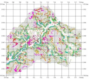
Figure 6. Deforestation prediction map based on Bayes probability
model performed better than the regression model. The regression model was able to identify about half of the deforestation areas at both training and prediction stages. In comparison, Bayes model successfully identified 53% and 60% of the deforestation area as training and validation, respectively (Table 2a). When the grid groups were reversed, the prediction rate of the Bayes model was also higher than the regression model. Though, the occurrence rate of the regression model was better than that of the Bayes model (Table 2b).
Although the accuracies of the 2 models were relatively close, the Bayes model may be more suitable for monitoring deforestation. Consistency was considered as a decisive measure especially when the prediction models were not significantly differed. The Bayes model demonstrated very consistent result. The differences between the occurrence and prediction rates were consistent in both half and systematic grid partitions.
Predicted deforestation map in the study
area based on the Bayes model (Table 2a) is shown in Figure 6. The pixels with the highest 10% estimated probability values were classified as the 0 to 10 % class, shown as red. The pixels of the next highest 10% classes were represented in orange, yellow, green and blue. Gray color was assigned to the remaining 50% percent of the area.
Factors of the probability model
There may be some factors that influence the performance of the Bayes model. The deforestation areas in Higashi-Shirakawa area during 1989 to 2001 was in fact the result of different land use decisions. The accuracy of prediction may be influenced by the heterogeneity of the deforestation areas and partition method of sub-areas.
Thresholding using 1 standard deviation from the mean as criterion may not adequately capture the heterogeneous nature i.e. various types and sizes of deforestation.
The Bayes model identified more than
70% of the deforestation areas for the top 30% of the study area. Even by visual interpretation of the deforestation area, it was difficult to identify areas such as discontinued and small patch type of deforestation in the Landsat TM of 2001.
Besides, there may be some changes in land cover during the time lag of 2 years between the satellite data and field work.
Difficulty in identifying deforestation for tea plantation establishment and agriculture road construction may be due to the time lag.
Ideally, the time of data acquisition should be synchronized. In practice, one can only make sure the data set is temporally as close as possible.
Conclusion
A quantitative model was proposed for predicting deforestation occurrence using PRC. The occurrence and prediction rates were expressed in terms of the distribution of deforestation pixel proportions corresponding to the unique combination of three geographic factors and one VCD factor. ORC and PRC based on the Bayes probability was useful for identify deforestation area. The systematic grid partition was the best spatial partition approach for constructing the Bayes model.
At a regional or national scale, geographic attribute information can be obtained with relative ease, either through digitizing of map sources or satellite data analysis. For improving the deforestation prediction, other factors such as stand structure may need to be considered. Further examination of the categorization of the factors may be needed.
It is believed that this new approach is comparable to other prediction models analyzing the causal factors of LULUCF.
Similar prediction model can also be constructed for monitoring other activities under the Kyoto Protocol such as afforestation and reforestation. We hope that the prediction model proposed in our study will contribute to the implementation process of the Kyoto Protocol.
REFERENCES
Bayes, T.1763. An essay towards solving a problem in the doctrine of chances.
Philosophical Transactions pp.376-398.
Carrera, A., M. Cardinali, R. Detti, F. Guzzetti, V. Pasqui and P. Peichenbach. 1991. GIS techniques and statistical models in evaluating landslide hazard. Earth surface processes and land forms pp.427-445.
Chung, C.F. and A.G. Fabbri. 1999.
Probabilistic prediction models for landslide hazard mapping. Photogrammeric engineering and remote sensing 65(12):1389-1399.
Chung, C.F. and A.G. Fabbri. 2003. Validation of spatial prediction model for landslide hazard mapping. Natural hazard 30:451-472.
Chung, C.F., A.G. Fabbri and C.J. Van Western. 1995. Multivariate regression analysis for landslide hazard zonation, Geographical information systems in assessing natural hazardsCarrara, A. and Guzzetti, F., editors.. kluwer academic publishers. Dordrecht, The Netherlands pp.107-133.
Eastman, J.R. and J.E. McKendry. 1991.
Change and time series analysis: Exploration in geographic information system technology, volume 1.
Elmore, A. J., J. F. Mustard, S. J. Manning and D. B. Lobell. 2000. Quantifying
vegetationchange in semiarid environments:
Precision and accuracy of spectral mixture analysis and the normalized difference vegetation index. Remote sensing of environment 73: 87-102.
Fabbri, A.G. and C.F. Chung. 1996. Predictive spatial data analysis in the geosciences, Spatial analytical perspectives on GIS in the environmental and socio-economic sciences, GIS DATA series 3,Taylor & Francis, London pp.147-159.
Hori, S., H. Hayashi, M. Amano, M.
Matsumoto and Y. Awaya. 2002.
Development of ARD detection method using Remotely sensed data. Sinrin-Kousoku.
Japan forest technology association 197:1-7.
IPCC 2003. Good Practice Guidance for Land Use Land-Use Change and Forestry, 4.24, IGES, Japan. pp. 1-42.
Forestry Agency. 1998. A Survey on methods of socioeconomic evaluation and scientific management: Development of evaluation methods of forest functions. Forestry
Agency, Tokyo, Japan. pp. 115-168.
Kodani, E. 2003. Developing algorism for detecting afforestation, reforestation and deforestation of Kyoto Protocol with time series of LANDSAT TM images.
Proceedings of the 114th Conference of the Japanese Forestry Society 114:192pp.
Smith, J.A., T.L. Lin and L.J. Ranson. 1980.
The Lambertian assumption and Landsat data. Photogrammeric engineering and remote sensing 46:1183-1189.
Tucker, C.J. and E.L. Maxwell. 1976. Sensor design for monitoring vegetation canopies.
Photogrammeric engineering and remote sensing 42(11): 1399-1410.
UNFCCC 1997. Kyoto Protocol to the United Nations Framework convention on climate change, 3pp.
http://unfccc.int/resource/docs/convkp/kpeng.
UNFCCC 2001. The Marrakesh Accords and the Marrakesh Declaration.