http://dx.doi.org/10.7840/kics.2014.39B.10.629
CAN-Based Networked Control Systems: A Co-Design of Time Delay Compensation and Message Scheduling
NGUYEN Trong Cac, NGUYEN Xuan Hung°, NGUYEN Van Khang*
ABSTRACT
The goal of this paper is to consider a co-design approach between time delay compensation and the message scheduling for CAN-Based Networked Control Systems (NCS). First we propose a hybrid priority scheme for the message scheduling in order to improve the Quality of Service (QoS). Second we present the way to calculate the closed-loop communication time delay and then compensate this time delay using the pole placement design method in order to improve the Quality of Control (QoC). The final objective is the implementation of a co-design which is the combination of the compensation for communication time delays and the message scheduling in order to have a more efficient NCS design..
Key Words : Co-design, Networked Control Systems, Message scheduling, QoS, QoC
First Author :Hanoi University of Science and Technology, Hanoi, Vietnam,
° Corresponding Author:R&D department, UINT company, Saint Aubin, France,
논문번호:KICS2014-07-263, Received July 14, 2014; Revised October 11, 2014; Accepted October 11, 2014
Ⅰ. Introduction
The study and design of Networked Control Systems (NCS) based on CAN bus is a very important research area today because of its multidisciplinary aspect (Automatic Control, Computer Science, and Communication Network).
Today the current design objective is to consider a co-design between the designs of Automatic Control (QoC) and Communication Network (QoS) in order to have efficient control systems[1] .
This paper presents a co-design between the QoC of the controller based on time delay compensations and the QoS of the communication network based on the scheduling of messages (Medium Access Control (MAC) protocol) for CAN-based control systems.
The MAC protocol of the CAN bus is the type of CSMA/CA (Carrier Sense Multiple Access/Collision Avoidance). Nodes which have frames to transmit listen to the medium, when the medium is free, they
begin a medium access tournament by sending and comparing the ID (IDentifier) bits placed at the beginning of the frames. Each node has a unique ID which represents the priority of the frame sent by this node and which allows to do the medium access tournament. The tournament is done by a comparison bit by bit of the same rank among the IDs of the contending frames from the Most Significant Bit (MSB) to the Least Significant Bit (LSB). A bit 0 is a dominant bit and a bit 1 is a recessive bit. In a bit-by-bit comparison, a bit 0 overwrites a bit 1. Therefore the higher the priority is, the lower the ID value is. At the end of the tournament, the node which has the highest priority (i.e., the lowest ID value) is the unique winner allowed to send its frame. The losers must wait until the end of the frame transmission of the winner and begin a new medium access tournament.
Some works[1,2] have considered both the time delay compensation and the message scheduling based on LEF (Large Error First) algorithm in which each message is assigned a priority level according
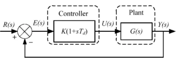
Fig. 1. Continuous control system.
Fig. 2. Time response y(t).
to the error value. The higher the error is, the higher the priority is and vice versa. A limitation of this paper is that the error value encoding is not bounded.
In the paper[3], the proposed time delay compensation is designed according to the dominant pole method and the message scheduling is based on the control signal u. The authors proposed a message scheduling scheme based on hybrid priority for CAN network using the standard 11 bit ID field where the ID field is divided into 2 small levels.
The level 1 (4 bits) represents a fixed priority and the level 2 (7 bit) represents a dynamic priority. A limitation of this study is to only use 4 bits for static priority, so they can determine a maximum number of 16 data flows (or nodes) which is not enough to address all nodes in a NCS.
The goal of this paper is to present a co-design to overcome the limitations analyzed above, which allows improving QoC and QoS simultaneously.
We use the tool TrueTime[4] for the simulation and the QoC evaluation. TrueTime is a toolbox based on Matlab/Simulink which allows simulating real-time network-based control systems.
This paper includes the following sections: the section II presents the context of the study; the section III presents the implementation of a hybrid priority scheme for message scheduling; the section IV presents the implementation of the compensation for communication time delays; the section V presents a co-design of time delay compensation and message scheduling; the conclusion is represented in the section VI.
Ⅱ. Context of the study
2.1 Process control application
The model of the considered process control application (using the Laplace transform) is given on Fig. 1.
The process to control is G(s)=1000/s(2s+1). The PD (Proportional Derivative) controller is PD=
K(1+sTd). The input reference is R(s) = 1/s (unity position step) and the output is Y(s). The phase margin of G(s) is 1.3° at the crossover frequency ωc
= 22.4 rad/s (i.e., the frequency such that
[5]. This phase margin is too small (the phase margin should be from 45° to 60°[6]). Here we consider that, initially, the PD controller must compensate a positive phase φc in order to have a system phase margin of 50°.
To do that, it must be:
(1)
We have K = 0.6598 and Td = 0.0509 s. The closed-loop transfer function is:
(2)
(3)
Where ωn is the natural pulsation (rad/s) and ζ is the damping coefficient.
We have =500Kand 2ζωn= 0.5+500KTd which give ωn = 18.16 rad/s and ζ = 0.48, the two poles p1,2 are p1,2= -ζωn± jωn
The settling time at 2% is ts = 382 ms, the
Fig. 4. Control system with time delays.
Overshoot is O = 38.17 %. The time response y(t) is represented in Fig. 2.
2.2 Implementation of a process control application on a CAN network
2.2.1 General model
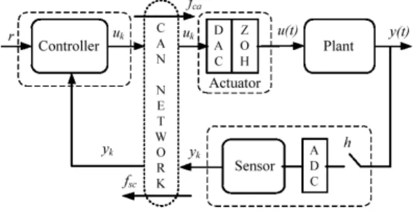
The general model of the implementation of a process control application through a CAN network is shown on Fig. 3.
The sensor receives the sampled output yk
provided by the Analog Digital Converter (ADC) and sends it to the controller via the CAN bus. The controller receives yk from the sensor, then calculates the control signal uk and sends uk to the actuator via the CAN bus. The actuator receives uk, converts uk into analog signal (u(t)) using the Digital Analog Converter (DAC) and then directly applies u(t) to the Plant. The Zero Order Hold (ZOH) keeps the value u(t) until the new sampling time.
We have two flows of frames: the Sensor-Controller flow which concerns the frames going from the sensor to the controller (noted fsc
flow and call “fsc frame” a frame of this flow); the Controller-Actuator flow which concerns the frames going from the controller to the actuator (noted fca
flow and call “fca frame” a frame of this flow). The sensor task is Time-Triggered while the controller and actuator tasks are Event-Triggered.
Fig. 3. Implementation of a process control application on a CAN network.
2.2.2 Sampling period
We call h the sampling period which is determined by considering the formula ωnh∈
[0.1;0.6][7]. Here we take h = 10 ms.
2.2.3 Communication time delays
Communication time delays in each sampling period consist of two components:
• The Sensor-Controller time delay concerns the transmission of fsc frames (noted τsc) which is the duration between the sampling instant (tk, k = 0, 1, 2…) and the reception instant of this frame by the controller. τsc includes the waiting time for medium access and the transmission time of a fsc
frame (noted Dsc).
• The Controller-Actuator time delay concerns the transmission of fca frames (noted τca) elapsed from the ready-to-send instant of the fca frame till the reception instant of this frame by the actuator. τca includes the waiting time for medium access and the transmission time of a fca
frame (noted Dca).
Note that the durations Dsc and Dca can be easily calculated by knowing the frame length and transmission speed.
The communication time delay of a closed-loop control system is:
(4) 2.2.4 NCS model with time delays
The model of the implementation of a process control application on a network can be represented by the continuous model given on Fig. 4 where a time delay τ is represented as e-τ.s
The transfer function F(s) is now:
(5)
The exponential function can be replaced with the Padé first order approximation i.e.,
(6) Fig. 5. Structure of the ID field.
Where
We get finally the transfer function in Equation (6). From Equation (6), we have 4 poles (3 poles p1, p2, p3 of the polynomial f3(s), p4 = −2/τca and 3 zeros (z1 = −1/Td, z2 = −2/τ, z3 = 2/τca).
2.3 Considered global control system
2.3.1 Control system setup
We implement 8 identical process control applications (noted P1, P2,…, P8) through a CAN network. So we have 24 different nodes connected through a CAN network and 16 data flows (8 fsc and 8 fca flows) sharing the network. We consider other parameters and conditions as followed: bit rate = 250 Kbit/s; data field length of a frame = 8 bytes, thus Dsc = Dca = 150 bits ; the sensor tasks are synchronous and have the same sampling period.
2.3.2 Priority of messages
Generally, the priorities are static priorities, i.e., each flow has a unique priority (specified a priori out of line) and all the frames of this flow have the same priority. In this work, we consider not only static priorities but also hybrid priorities (as we said in the introduction). The hybrid priority consists in structuring the field ID in two levels (Fig. 5) where the Level represents the uniqueness of the message (flow priority) which is a static priority and Level 2 represents the transmission urgency of the frame[9] . This concept has a great interest during the transient behavior of systems[10].
In the context of the competition based on these
hybrid priorities, the message scheduling is executed by comparing first the bits of the Level 2 (urgency predominance). If the urgencies are identical, the Level 1 (static priorities which have the uniqueness properties) resolves the competition.
2.2.3 Static priorities associated to the fsc and fca flows
Here we consider the conclusion shown in : The priority of the fca flow should be higher than the priority of the fsc flow in order to get the best results. Considering n process control applications (P1, P2,…, Pn), each process has one fsc flow and one fca flow. We call Prio_fca_i and Prio_fsc_i the priorities of the fsc and fca flows of the process Pi (i
= 1, 2,…, n), respectively. The priorities of 2n data flows are arranged in the following order: Prio_fca_1
> Prio_fca_2 > … > Prio_fca_n > Prio_fsc_1 >
Prio_fsc_2 > … > Prio_fsc_n.
2.2.4 Criteria of the QoC evaluation
The QoC is evaluated through a cost function ITSE (Integral of Time-weighted Square Error):
(7)
with T > ts in order to cover the transient regime duration. We consider T = 1000 ms and we get the value of J for the control system without network (section II-1) is J0 = 0.001962 which is considered as the reference value. The QoC criteria is represented by the term:
(8)
The smaller the value ∆J/J0 % is, the better the QoC is. We will also consider the time response for the QoC evaluation.
Ⅲ. The implementation of a hybrid priority scheme for message scheduling
3.1 Idea of hybrid priorities
The ID field into 2 small fields as represented in Fig. 5. Level 2 (m high significant bits) represents transmission urgency which is called dynamic priority part with its value ID_dyn. The ID_dyn can be changed during system operation and several data flows can share the same ID_dyn. Level 1 (n-m bits) which is called static priority part represents the uniqueness of data flows as its value ID_sta is fixed, unique and specified before system running. The uniqueness means that there are no two or more nodes having the same ID_sta. The term “hybrid priority” means the combination of dynamic priority and static priority. The idea of this ID field structure was first introduced in [10]. Then other studies[9,12]
also used the similar ID field structure. The medium access tournament is done firstly by comparing Level 2. If there are several data flows having the same ID_dyn, Level 1 will determine the only winner allowed to access to the medium.
3.2 Specifying of the dynamic priority
Specifying dynamic priority part requires, firstly, to determine QoC parameter of the process control application which gives information on the transmission urgency, and secondly, to translate these urgencies into dynamic priorities (i.e., computation of dynamic priorities).
Two main QoC parameters using for representing the transmission urgency are steady state error error e[2,12] and control signal u[3,9]. Some other works use the deadline[10,13]. With these parameters, the authors proposed different functions for computation of dynamic priorities. The principle is that the higher the values of e, u or deadline are, the higher the
dynamic priorities are.
Concerning the works using the error e, they used an extended ID field of 29 bits (16 bits for ID_dyn and 10 bits for ID_sta). The value of e is encoded directly into the ID_dyn value. The first limitation is that, we have a wide range of error value and this is not bounded (for example when the system is unstable, the error is infinite). Mapping these error values in a definite number of priority bits is not an easy task. The second limitation is that, they assume the existence of a master node knowing the current states of all controller nodes. Maintaining a global state in the whole distributed control system can be problematic.
The works using the control signal u have overcome the unbounded value by a saturation value us (if u is higher than us, the dynamic priority is maximum). They used a standard ID filed of 11 bits (7 bits for ID_dyn and 4 bits for ID_sta). So, they can determine a maximum number of 16 data flows (or nodes) which is not enough to address all nodes in a NCS.
3.3 Proposal
3.3.1 A. ID field
We use an extended ID field of 29 bits with 11 bits for dynamic priority part, and 11 bits for static priority part. That overcomes the limitation concerning number of ID_sta bits.
3.3.2 Control parameters
Both the error e and the control signal u are used for making the dynamic priority.
3.3.3 Computation of dynamic priorities The dynamic priority (noted Prio_dyn) is calculated by the controller using functions represented in Fig. 6 and Equations (9 & 10) where emax and umax are the maximum values of e and u respectively when we consider the initial continuous control system without the network.
(9)
Fig. 6. Functions of e and u.
Fig. 7. Implementations of process control applications on a CAN network.
(10)
3.3.4 Encoding priority into ID field
The dynamic priority part consists of 11 bits which is able to represent 211 = 2048 priority levels from 0 to 2047. The minimum dynamic priority is Prio_dynmin = 0 corresponding to the ID_dyn of 11 recessive bits (bit 1). The maximum dynamic priority is Prio_dynmax = 2047 corresponding to the ID_dyn field of 11 dominant bits (bit 0). The relation between the ID_dyn and the Prio_dyn is as follows:
(11) 3.3.5 Implementation of the hybrid priority scheme
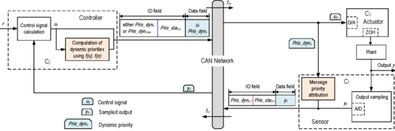
Before we present how the hybrid priority scheme works, we should consider the implementation of a process control application on the CAN network as represented on Fig. 7.
Now, we can see how the hybrid priority works.
Firstly, concerning the static priority part, this priority of each node is specified before the system running. The subsection II-3C shows that we have to set static priority of the fca flow (noted Prio_stafca) higher than that of the fsc flow (noted Prio_stafsc) in order to get the best results.
Here we will consider this conclusion. Secondly, concerning dynamic priority part, its implementation is as follows:
• At the instant tk, the sensor samples the output (yk) and gets dynamic priority (Prio_dynk-1) sent from the controller in the previous period (i.e., period starting at tk-1). After that, the sensor uses this priority (Prio_dynk-1) to send its frame (containing yk) to the controller.
• After receiving the fsc frame sent from the sensor, the controller computes the control signal uk and the dynamic priority Prio_dynk (by equations (9
& 10) and sends its frame on the network. Then, the actuator will get uk and apply it to the controlled plant, while the sensor will get Prio_dynk to use in the next sampling period (period starting at tk+1).
Concerning dynamic priority using to send the fca
frame by the controller, there are two ways: the first one is that the controller use the Prio_dynk value which has just been computed[9]; and the second one is to use the Prio_dynmax[2,3]
. It is evident that the second way ensures that fca frame will be sent immediately after the reception of fsc frame (computational time delays in the controller is
P1 P2 P3 P4 P5 P6 P7 P8
Static priority scheme 1.2 2.4 3.6 4.8 6.0 7.2 8.4 9.6 8.4
Hybrid priority scheme with e 3.67 4.24 4.73 5.29 5.86 6.21 6.49 6.71 3.04
Hybrid priority scheme with u 4.73 4.87 5.01 5.58 5.65 5.51 5.79 6.07 1.34
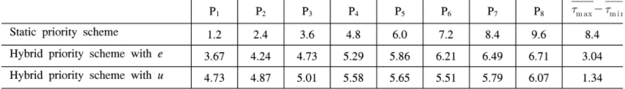
Table 2. QoS (ms).
negligible). Therefore, comparing to the first way, the second way performs a shorter time delay of the closed loop.
In this paper, we consider the second one, i.e. the controller uses the Prio_dynmax to send its frames.
Noting that, at the instant 0 (t0 = 0), the sensor has no information about the dynamic priority from the controller. Therefore we consider that the sensor uses, at the first time, the Prio_dynmax.
3.4 Implementation of process control application on CAN network
3.4.1 Criteria of the QoS evaluation
In order to evaluate the QoS, we calculate first the communication time delay τi of the closed loop control system in each sampling period starting at ti
according to the Equation (4), then we compute the average value of theses time delays during the settling time ts by the following formula:
(12)
Where n is the number of sampling period in the settling time. The smaller the value is, the better the QoS is.
3.4.2 Criteria of the QoC evaluation
We use the criteria ITSE in the Equations (7 & 8).
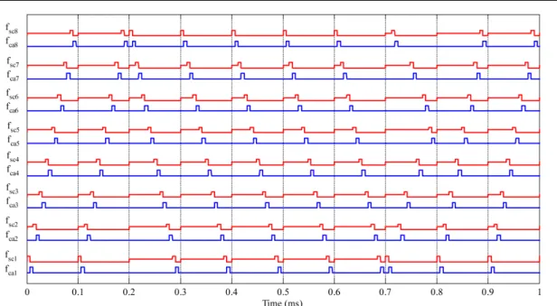
3.4.3 Results
• Quality of Service (QoS)
We present the QoS in term of of the 8 processes on Table 2 and the scheduling of frames in the first 10 sampling periods on Fig. 9a, 9b and 9c (in which fcai and fsci are the controller-actuator frame and sensor-controller frame of the process i).
For static priority scheme, the process with higher
priority has smaller time delay (Table 2 and Fig.
9a). We see that P1 has the highest priority so its delay is the smallest while P8 has the lowest priority so its delay is the biggest. The frame exchanges are identical for all periods (Fig. 9a). The protocol based on static priority is called deterministic protocol.
For the hybrid priority scheme (with e and u), we obtain time delays more balanced than these with static priorities (Table 2). The frame exchanges are not identical in each sampling period (Fig. 9b, Fig.
9c) due to the predominant role of the parts
“dynamic priority” which make the priority changed in each sampling period.
The QoS balance can be observed by the difference between the maximum delay and the minimum delay in each priority scheme in Table 2.
We see that these differences are small with hybrid priorities (3.04 ms with e and 1.34 ms with u) while this value is very big with static priorities (8.4 ms).
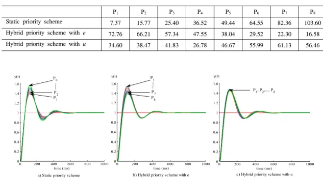
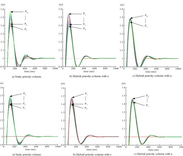
• Quality of Control (QoC)
The QoC is represented on the Table 3 (ΔJ/J0 %) and Fig. 8 (time responses y(t)). We see also the balances of QoC with hybrid priorities compared with static priorities. It is logical because balances of QoS induce balances of QoC. The conclusions of QoC for different priority schemes are similar to these of QoS.
Precisely, for the static priority scheme, the higher the priority is, the better the QoC is, and for the hybrid priority schemes, the QoCs are more balanced than these of the static priority scheme.
Note that the hybrid priority allows more balanced QoCs between processes than the static priority but the best QoC and the worst QoC belong to the static priority. The advantage of the hybrid priority is that if we have a QoC threshold which
P1 P2 P3 P4 P5 P6 P7 P8
Static priority scheme 7.37 15.77 25.40 36.52 49.44 64.55 82.36 103.60
Hybrid priority scheme with e 72.76 66.21 57.34 47.55 38.04 29.52 22.30 16.58 Hybrid priority scheme with u 34.60 38.47 41.83 26.78 46.67 55.99 61.13 56.46 Table 3. QoC (Δ J/J0 %).
0 200 400 600 800 1000
0 0.2 0.4 0.6 0.8 1 1.2 1.4 1.6
time (ms) y(t)
0 200 400 600 800 1000
0 0.2 0.4 0.6 0.8 1 1.2 1.4 1.6
time (ms) y(t)
0 200 400 600 800 1000
0 0.2 0.4 0.6 0.8 1 1.2 1.4 1.6
time (ms) P8 y(t)
P1 P2
P1
P7 P8
P1, P2,..., P8
a) Static priority scheme b) Hybrid priority scheme with e c) Hybrid priority scheme with u
Fig. 8. Time responses.
a) Static priority scheme: message exchanges in the first 10 sampling periods.
can not to be exceeded, the hybrid priority scheme allows implementing more applications on the network than the static priority scheme. For example if the QoC threshold is 80%, we can implement all 8 processes with the hybrid priority but only 6 processes with the static priority (see Table 3).
Ⅳ. The Implementation of the Compensation for Communication Time
Delays 4.1 Ideas
The QoS considered is the closed-loop
b) Hybrid priority scheme (parameter e): message exchanges in the first 10 sampling periods.
c) Hybrid priority scheme (parameter u): message exchanges in the first 10 sampling periods.
Fig. 9. Message exchanges in the first 10 sampling periods.
communication time delay during each sampling period. With the knowledge of τ, the controller can compensate this time delay by modifying the parameters K and Td in such a way to maintain the same type of transient behavior for the process control application as before the implementation on
the network. As the transfer function of the system implemented on the network, the modification of K and Td, according to the pole placement design method, must keep the main role for the 2 poles p1,2
which are called the dominant poles and integrate the conditions which give an insignificant role to the
poles p3, p4 (called insignificant poles). Actually, the numerator of Equation (6) has now three zeros. Thus we have to evaluate the influence of these zeros on the overshoot.
4.2 Proposal
4.2.1 Computation of closed-loop communication time delays
The computation of closed-loop communication time delays is done by the controller in each sampling period.
Concerning the time delay τsc, as the controller has the knowledge of sampling instants tk (k = 0, 1,…), it can easily deduce the value of τsc by the time difference between the reception instant of fsc
frames and tk. Concerning the time delay τca, it cannot be calculated because the fca frames have not been transmitted yet. However, due to the hypotheses in subsection II-3B (i.e., the priority of the controller is higher than this of the sensor; there is no competition between the controllers; there is no data lost), the controller can immediately send its frame. Therefore, τca is equal to the duration of a frame transmission (Dca). The closed-loop time delay will be computed by the controller as followed:
τ = τsc+ Dca (13)
4.2.2 Time delay compensation steps
The compensation for time delays done by the controller in each sampling period has the following steps:
• Step 1: Identifying expected poles including the dominant poles and the other poles which are selected equally to the real part of the dominant pole divided α, with α= 2 ÷ 10[7].
• Step 2: Computing communication time delayτ.
• Step 3: Computing the controller parameters according to the time delay value in order to maintain the position or the value of the expected poles.
• Step 4: Computing the control signal based on the new control parameters calculated in the previous step.
4.3 The computations in the controller for the maintenance of the pole placement design method
Consider the polynomial f3(s) in the denominator of Equation (6), this polynomial concerns the poles p1, p2, p3 and can be written as:
(14)
By identifying f3(s) with Equation (14), we get the relations which allow determining the values of p3, K and Td:
(15)
We replace the value of K in Equation (6) by this one found in Equation (15), we have now the transfer function F(s):
(16)
Note that p3 and p4 = −2/τca are real poles.
4.4 Conditions for the insignificance of the poles p3 and p4
We take the conditions expressed by [5] i.e., the real part is five times smaller than the real part of the dominant poles, then:
• p3 ≤ 5R which need τsc + τca < 26.08 ms.
• p4 ≤ 5R which need τca < 45.87 ms.
These conditions are always satisfied as the sampling period h is 10 ms and τsc + τca is always smaller than h.
4.5 Effect of the zeros
“When a zero gets closer to the origin, the overshoot increases”[14,15]. For a negative zero (call z0 the absolute value of this zero), in [14], the zero
τca (ms) τ (ms) K Td (s) p1,2 p3 p4 O (%) z1 z2 z3
1 2 0.6372 0.0533 -8.72 ± j15.93 -966 -2000 32.15 -18.7 -1000 2000
2 3 0.6260 0.0544 -8.72 ± j15.93 -633 -1000 33.73 -18.4 -667 1000
3 4 0.6148 0.0554 -8.72 ± j15.93 -466 -667 35.46 -18.1 -500 667
Table 4. Validation of the pole placement design method, τsc = 1 ms.
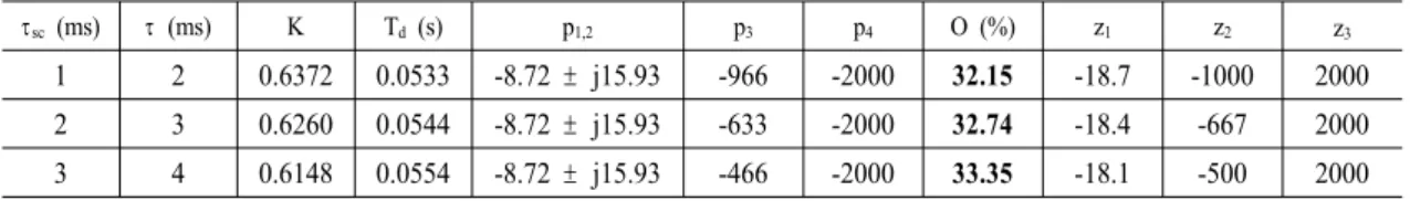
τsc (ms) τ (ms) K Td (s) p1,2 p3 p4 O (%) z1 z2 z3
1 2 0.6372 0.0533 -8.72 ± j15.93 -966 -2000 32.15 -18.7 -1000 2000
2 3 0.6260 0.0544 -8.72 ± j15.93 -633 -2000 32.74 -18.4 -667 2000
3 4 0.6148 0.0554 -8.72 ± j15.93 -466 -2000 33.35 -18.1 -500 2000
Table 5. Validation of the pole placement design method, τca = 1 ms.
has a little effect and can be neglected if . For a positive zero (call z0 the value of this zero), in [15], the overshoot is evaluated as follows:
(17)
Where . We see that if
, the overshoot can be re-written as i.e., we have the overshoot of the second order system without zero.
We can thus consider that if and (these conditions induce that z0 > 87.17 (with ωn = 18.16, ζ = 0.48)).
We consider now the three zeros:
• The negative zero z2 = −2/τ : as τ = τsc + τca
is smaller than h, z2 is smaller than −2/0.01 =
−200. We see that . Thus the zero z2 can be neglected.
• The positive zero z3 = 2/τca: because of τca is smaller than h, z3 is bigger than 2/0.01 = 200, thus z3 > 87.17. Hence the zero z3 can be neglected.
• The negative zero z1 = −1/Td: note that this zero is based on a parameter of the controller (Td). The effect of z1 depends on the value of Td; the higher the value of Td is, the more closed the zero is to the origin, thus the zero
has the stronger effect.
Remark about the transfer function after the compensation of the time delay: Considering the insignificance of the poles p3, p4 and the negligible effect of the zeros z2 and z3, the transfer function in Equation (16) can be written as Equation (18).
(18)
We see that we have the same form as the transfer function of the system without delays in Equation (3), but the value of Td is now changed.
4.6 Validation of the pole placement design method
Table 4 and Table 5 show the results obtained by considering different loop delays τ.
We see that the dominant poles are maintained which results from the action on K and Td (decrease of K and increase of Td).
We also see the increase of the overshoot (mainly due to the increase of the zero z1 = −1/Td; the role of the zeros z2, z3 and of the poles p3, p4 is negligible)
4.7 Considering the implementation of the 8 process control applications
We want to show here the interest of the pole placement design method (which is based on an adaptive controller i.e. the parameters of the controller are modified according to the closed-loop
a) Non-Compensation
b) Compensation for Communication time delay Fig. 10. Time responses of the 8 applications.
communication time delays) in comparison with the case where we do not use this method (i.e., we have a fixed controller). The comparison between the case adaptive controller (i.e., compensation) and the case fixed controller (i.e., non-compensation) is presented on and on Fig. 10 (time responses y(t)).
From the results of the case non-compensation:
the performances follow the order of the priorities which is normal (lower is the priority, then higher is the time delay and less good is the performance).
From the results of the case compensation for communication time delay: it improves the results (what was waited for!) which are less dispersed (the influence of the priorities is reduced); however we cannot have identical performances for all the process control applications because of the effect of the zero −1/Td (as the applications which have less priority have higher delays, the compensation requires higher values of Td which induces that the zero −1/Td moves closer to the origin).
We note also the effect of the zero −1/Td by the increase of O (Fig. 10 (b)) compared with the O (secction II-1) of the control system without network.
Ⅴ. A Co-Design of Time Delay Compensation and Message Scheduling
5.1 Ideas
The idea is to combine the frame scheduling scheme based on the hybrid priority and the method of compensation for communication time delay in order to have a more efficient NCSs. However, concerning the close-loop time delay compensation, in the sampling period k, we cannot consider here that the controller can use the value of the close-loop communication time delay of the sampling period (k-1) because now, taking into account for the dynamic priority used by the sensor task, the time delay (τsc + τca) changes every period.
Then the controller must make the delay compensation in the sampling period k by knowing the close-loop communication time delay of this sampling period k. We explain now this implementation.
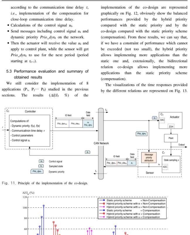
5.2 Principle of the implementation of the co-design
This principle, relatively to the sampling period starting at tk, is represented on Fig. 11 where we indicate the content of the fsc and fca frames and the computations done by the controller.
The process of co-design implementation in each cycle starting at tk as follows: Sensor sampling state variables x and receive priority value sent from the controller in the previous period (period starting at tk-1), then use the sensor priority this (Prio_dynk-1) to send a message containing xk to the controller.
The controller after receiving the signal from the sensor xk, will perform the following steps:
• The computations of dynamic priority Prio_dynk based on the function f(u) and f(e) (by Equations (9 & 10).
• Calculations of close-loop communication time delay τ and the parameters of the controller
Fig. 11. Principle of the implementation of the co-design.
0 20 40 60 80 100 120 ΔJ/J0 (%)
Static priority scheme + Non-Compensation Hybrid priority scheme with e + Non-Compensation Hybrid priority scheme with u + Non-Compensation Static priority scheme + Compensation Hybrid priority scheme with e + Compensation Hybrid priority scheme with u + Compensation
P1,..., P8 P1,..., P8 P1,..., P8 P1,..., P8 P1,..., P8 P1,..., P8
Fig. 12. Graphic representation of the QoC (Δ J/J0 %) of the 8 applications.
according to the communication time delay τ, i.e., implementation of the compensation for close-loop communication time delay.
• Calculations of the control signal uk.
• Send messages including control signal uk and dynamic priority Prio_dynk on the network.
• Then the actuator will receive the value uk and apply to control plant, while the sensor will get Prio_dynk to use for the next period (period starting at tk+1).
5.3 Performance evaluation and summary of obtained results
We still consider the implementation of 8 applications (P1, P2… P8) studied in the previous sections. The results (ΔJ/J0 %) of the
implementation of the co-design are represented graphically on Fig. 12, obviously show the balanced performances provided by the hybrid priority compared with the static priority and by the co-design compared with the static priority scheme (compensation). From these results, we can say that, if we have a constraint of performance which cannot be exceeded (not too small), the hybrid priority allows implementing more applications than the static one and, extensionally, the bidirectional relation co-design allows implementing more applications than the static priority scheme (compensation).
The visualizations of the time responses provided by the different relations are represented on Fig. 13.
0 200 400 600 800 1000 0.9
1 1.1 1.2 1.3 1.4 1.5 1.6
time (ms) y(t)
0 200 400 600 800 1000
0.9 1 1.1 1.2 1.3 1.4 1.5 1.6
time (ms) y(t)
0 200 400 600 800 1000
0.9 1 1.1 1.2 1.3 1.4 1.5 1.6
time (ms) y(t)
P8
P1 P8
a) Static priority scheme b) Hybrid priority scheme with e c) Hybrid priority scheme with u
P1
P7 P8 P2
P1
0 200 400 600 800 1000
0.9 1 1.1 1.2 1.3 1.4 1.5 1.6
time (ms) y(t)
0 200 400 600 800 1000
0.9 1 1.1 1.2 1.3 1.4 1.5 1.6
time (ms) y(t)
0 200 400 600 800 1000
0.9 1 1.1 1.2 1.3 1.4 1.5 1.6
time (ms) y(t)
P1 P8
P1 P8
P2
P8 P7 P1
c) Hybrid priority scheme with u a) Static priority scheme b) Hybrid priority scheme with e
Fig. 13. Zoom time responses (top: without co-design (zoom of Fig. 8); bottom: co-design).
Ⅵ. Conclusions
In this paper, we have presented a co-design between the time delay compensation and the message scheduling which have the following advantages. First, this co-design overcomes the limitations of related works discussed in Section I (bounded error value, limited number of network nodes). And second, this co-design allows improving simultaneously the QoC and the QoS of CAN-based NCSs. More precisely, by the hybrid priority, we have balance aspect compared with the static priority and by the delay compensation, we maintain the balanced aspect while improving the QoC. The results obtained also allow considering the possibility to implement more applications than with the static priority.
References
[1] Ye-Qiong Song, “Networked Control Systems:
From independent designs of the network QoS and the control of the co-design,” 8th IFAC Int. Conf. Fieldbuses Netw. Ind. Embedded Syst., pp. 155-162, Seoul, Korea, May 2009.
[2] P. Martí, J. Yépez, M. Velasco, R. Villà and J. M. Fuertes, “Managing Quality-of-Control in network-based control systems by controller and message scheduling co-design,” IEEE Trans. Ind. Electron., vol 51, no. 6, pp.
1159-1167, Dec. 2004.
[3] Xuan Hung Nguyen and G. Juanole, “Design of Networked Control Systems on the basis of interplays between Quality of Control and Quality of Service,” 7th IEEE Int. Symp. Ind.
Embedded Syst., pp. 85-93, Karlsruhe, Germany, Jun. 2012.
[4] M. Ohlin, D. Henriksson, and A. Cervin,
“TrueTime 1.5 - Reference Manual,” Lund Inst. Technol., Sweden, 2007.
[5] F. Golnaraghi and Benjamin C. Kuo, Automatic Control Systems, 8th Ed., NY: John Wiley &
Sons, INC, pp. 236-245, 2003.
[6] John J. D’Azzo and C. H. Houpis, Linear Control System Analysis and Design:
Conventional and Modern, 4th Ed., NY: McGraw- Hill, 1995.
[7] Karl J. Åström and B. Wittenmark, Computer controlled systems: theory and design, 3th Ed., NJ: Prentice Hall, 1997.
[8] S. Hasnaoui, O. Kallel, R. Kbaier, and S. Ben Ahmed, “An implementation of a proposed modification of CAN protocol on CAN fieldbus controller component for supporting a dynamic priority policy,” 38th Ann. Meeting of the Ind. Appl. Conf., pp. 23-31, vol 1, Salt Lake, USA, Oct. 2003.
[9] G. Juanole and G. Mouney, “Networked Control Systems: Definition and analysis of a hybrid priority scheme for the message scheduling,” 13th IEEE Conf. Embedded and Real-Time Comput. Syst. Appl.(RTCSA 2007), pp. 267-274, Daegu, Korea, Aug. 2007.
[10] K. M. Zuberi and K. G. Shin, “Scheduling messages on Controller Area Network for real time CIM applications,” IEEE Trans. Robot.
Autom, vol 13, no. 2, pp. 310-316, Apr. 1997.
[11] G. Juanole, G. Mouney, C. Calmettes, and M.
Peca, “Fundamental considerations for implementing control systems on a CAN network,” 6th Int. Conf. Fielbus Syst. and their Appl., pp. 280-285, PUE, Mexico, Nov.
2005.
[12] M. Velasco, P. Martí, R. Castané, J. Guardia and J. M. Fuertes, “A CAN application profile for control optimization in Networked Embedded Systems,” 32nd Ann. Conf. IEEE Ind. Electron., pp. 4638-4643, Paris, France, Nov. 2006.
[13] Gregory C. Walsh and Hong Ye, “Scheduling
of Networked Control Systems,” IEEE Control Syst. Mag., vol 21, no. 1, pp. 57-65, Feb.
2001.
[14] R. C. Dorf and R. H. Bishop, Modern control systems, 10th Ed., NJ: Prentice Hall, 2005.
[15] Byung-Moon Kwoon, Hee-Seob Ryu, and Oh-Kyu Kwo, “Transient response analysis and compensation of the second order system with one RHP real zero,” Trans. Control, Autom. Syst. Eng., vol 2, no. 4, pp. 262-267, Dec. 2000.
NGUYEN Trong Cac
He is a Ph.D. student in Hanoi University of Science and Technology (HUST), Vietnam, where he has been since 2011.
He received M.Sc. degree from the HUST in 2005. From 2006 until now he has been working at Saodo University, Vietnam.
Areas of interest: Industrial Informatics and Embedded Systems, Networked Control Systems (NCS).
NGUYEN Xuan Hung
June 2007 : Engineer degree in Industrial Informatics from Hanoi University of Science and Technology (HUST), Vietnam.
June 2008 : Master degree in Automatic Control from Institut National Polytechnique de Grenoble (INPG), France.
Dec 2012 : PhD degree in Embedded Systems from nstitut National des Sciences Appliquées de Toulouse (INSA), France.
2013 : R&D Engineer at Atomic Energy and Alternative Energies Commission (CEA), Grenoble, France.
Jan 2014 to present : R&D Engineer at UINT company, France.
Areas of interest : Industrial communication, Embedded Systems, Networked Control Systems.
NGUYEN Van Khang
He is a Assoc. Professor in Hanoi University of Science and Technology (HUST), Vietnam, where he has been since 2010.
He received Dr. degree from the HUST in 1997. From 1998 until now he has been working at HUST.
Areas of interest : Industrial Informatics and Embedded Systems, Industrial Electronics, Distributed Control Systems, Networked Control Systems (NCS).