http://dx.doi.org/10.7848/ksgpc.2015.33.4.259
이종 공간 데이터를 활용한 에지 정보 기반 도시 지역 변화 탐지
Urban Change Detection Between Heterogeneous Images Using the
Edge Information
오재홍1) · 이창노2) Oh, Jae Hong · Lee, Chang No
Abstract
Change detection using the heterogeneous data such as aerial images, aerial LiDAR (Light Detection And Ranging), and satellite images needs to be developed to efficiently monitor the complicating land use change. We approached this problem not relying on the intensity value of the geospatial image, but by using RECC(Relative Edge Cross Correlation) which is based on the edge information over the urban and suburban area. The experiment was carried out for the aerial LiDAR data with high-resolution Kompsat-2 and –3 images. We derived the optimal window size and threshold value for RECC-based change detection, and then we observed the overall change detection accuracy of 80% by comparing the results to the manually acquired reference data.
Keywords : Change Detection, Edge Information, RECC, LiDAR, High-resolution Satellite Images
초 록
국토 공간 활용이 복잡해짐에 따라 항공사진, 항공 라이다, 위성영상 등 국토 공간에 대한 정보를 효율적으로 취 득하고 분석하기 위한 이종 데이터간의 변화 탐지 기법의 개발의 필요성이 증대되었다. 따라서 본 연구에서는 도
시 및 주변 지역에 대하여 취득된 이종 데이터간의 변화 탐지를 위해 화소값에 기반하지 않고 에지 정보에 기반한
RECC (Relative Edge Cross Correlation)기법을 제안하였다. 항공 라이다와 고해상도 위성영상인 아리랑 2호 및 3 호 영상에 대한 실험을 통해 변화 탐지 결과를 분석하여 RECC를 위한 적정 윈도우 크기 및 임계 계수를 도출하였
고, 육안 분석을 통해 획득한 레퍼런스 데이터와의 비교를 통해 약 80%의 정확성을 보임을 확인할 수 있었다.
핵심어 : 변화 탐지, 에지 정보, RECC, 라이다, 고해상도 위성영상
259 Original article
Received 2015. 06. 24, Revised 2015. 07. 26, Accepted 2015. 08. 07
1) Member, Dept. of Civil Engineering, Chonnam National University (E-mail: [email protected])
2) Corresponding Author, Member, Dept. of Civil Engineering, Seoul National University of Science and Technology (E-mail: [email protected]) This is an Open Access article distributed under the terms of the Creative Commons Attribution Non-Commercial License (http://
creativecommons.org/licenses/by-nc/3.0) which permits unrestricted non-commercial use, distribution, and reproduction in any medium, provided the original work is properly cited.
1. 서 론
국토 공간을 효율적으로 관리하고 분석하기 위해서 항공사 진 등 공간 데이터가 주기적으로 획득되고 있으며, 이렇게 원 격에서 얻어지는 다양한 공간 데이터는 현장 자료 수집에 비 해 비용을 절감시킬 수 있을 뿐 아니라 대상지에 대한 종합적
인 분석을 가능케 하여 환경 변화, 도시 변화 분석 및 매핑에 널리 활용되고 있다. 공간 데이터를 이용한 변화 분석을 위해 활용되는 변화 탐지 기술은 다중 시간대에 걸쳐 얻어지는 공 간 데이터를 이용하여 변화된 지역을 자동으로 검색해주는 기술로서, 작업자로 하여금 변화지역을 쉽게 인지하게 도와주 거나 변화 지역을 매핑하고 정량화하는데 필수적인 기술이다.
Journal of the Korean Society of Surveying, Geodesy, Photogrammetry and Cartography, Vol. 33, No. 4, 259-266, 2015
260
Fig. 1. LiDAR image preparation from the point cloud 특히 국토 공간 활용이 복잡해짐에 따라 항공사진, 항공 라이
다, 광학 위성영상, 레이더 영상 등 공간 데이터의 종류가 보다 다양화 되었고, 이에 따라 이종 데이터간의 변화 탐지 기법의 개발의 필요성이 증대되었다.
공간 영상 정보를 이용한 변화 탐지의 일반적인 과정은 기 하보정 및 방사보정, 선정된 알고리즘에 따른 변화 탐지, 그리 고 변화 탐지 정확도 검사 과정으로 마무리된다. 변화 탐지를 데이터의 종류에 따라 구분해 보면 중저해상도 위성데이터, 레이더 데이터, 항공사진, 수치지도, 항공 라이다 데이터 등으 로 나뉠 수 있으며, 변화 탐지 기법에 따르면 차분에 의한 기 법 및 피복 분류를 통한 비교 기법 (Maas, 1999; Song et al., 2001; Deng et al., 2009), 분광 벡터 분석 기법 (Chen et al., 2003; Zhang et al., 2009), 객체 지향 기법 (Chen et al., 2012) 등으로 나뉠 수 있다.
변화 탐지 기법의 문제점은 앞서 언급한 데이터 및 기법에 상관없이 공통적으로 나타난다. 첫 번째 문제점은 두 시기 데 이터 간의 정확한 상호좌표등록(co-registration)을 필요로 한 다는 것이다. 즉, 대부분의 변화 탐지 기법들은 다시기 데이터 에서 동일한 위치의 화소값을 비교 분석하기 때문에 좌표등 록에서 발생하는 오차는 변화탐지 결과의 오류로 직결된다.
두 번째 문제점은 상호좌표등록이 정확히 이루어졌다 하더라 도 동일 위치의 공간 영상 화소값 패턴이 달라질 수 있다는 점 에 있다. 대상물의 분광학적 특성을 기록하는 공간 영상의 특 성상 촬영 시간, 센서 보정 정도, 대기 상태, 그림자 등으로 인 해 동일한 지역이라 하더라도 동일한 밝기값을 기대하기는 어 렵다 (Chen et al., 2005). 이질적인 특성을 나타내는 공간 영 상을 이용하여 변화 탐지를 수행하기 위해서는 언급한 좌표 등록 오차와 분광 특성의 차이에 민감하지 않은 기법의 적용 이 필요하다.
따라서 본 연구에서는 라이다 데이터와 광학 영상의 조합 과 같이 공간 영상의 특성, 특히 분광정보의 차이가 현격히 나는 조합을 대상으로 변화 탐지를 적용하기 위해, 분광정보 를 이용하지 않고 대상지 지형 및 지물 형상의 에지 정보를 이 용하는 RECC (Relative Edge Cross Correlation) 기법 (Oh et al., 2012; Lee and Oh, 2014)을 적용하여 분석해 보았다.
RECC는 상관계수 매칭과 동일한 형태를 나타내지만 이진 (binary) 형태의 에지 정보를 이용한다는 차이가 있으며, 원 래는 이종 영상간의 에지 매칭을 위해 개발된 유사도 계산 연 산자이다. 그러나 변화가 많이 존재하는 지역의 경우 RECC 기법이 비유사성을 나타내는 인자로 활용될 수 있으므로, 변 화 탐지에 적용 가능성을 분석해 보고자 하였다. 본 논문에 서는 항공 라이다와 고해상도 위성영상인 아리랑 2호 및 3호
영상에 RECC 기법을 적용하여 RECC 윈도우 크기 및 임계 값 설정에 대한 실험을 수행하고, 참조 데이터를 통한 변화 탐 지 정확도를 분석하여 RECC 기법의 적용 타당성에 대해 알 아보고자 하였다.
본 논문의 구성은 아래와 같다. 2장에서는 방법론을 제시 하였다. 3장에서는 항공 라이다 데이터와 아리랑 2호 및 3호 영상을 이용한 실험 결과 및 분석을 제시하였고, 마지막 4장 에서 결론을 제시하였다.
2. 방법론
2.1 영상 준비
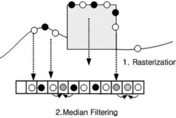
라이다의 경우 포인트 클라우드의 형태로 되어 있어 이 를 변화 탐지를 위한 영상 형태로 변환한다. 이 때 두 가지 영상을 생성하는데, 하나는 표고값을 이용한 DEM (Digital Elevation Model)이고, 두 번째는 반사강도 값을 이용한 반사 강도 영상이다. 두 영상 모두 동일한 방법으로 생성될 수 있 다. 즉, 라이다 데이터는 3차원 좌표값으로 표현되어 있으므 로, 라이다 데이터의 표고값이나 반사강도값 (intensity)만을 해당 수평위치에 래스터화하면 된다. Fig. 1과 같이 정해진 공 간 해상도의 영상 격자를 생성하고, 라이다 포인트가 해당하 는 격자에 표고 또는 반사값을 저장하여 영상을 제작하는 간 단한 과정이다.
이 때 두 가지를 고려해야 하는데, 첫 번째는 동일 격자에 여러 라이다 포인트가 존재할 수 있고, 두 번째는 건물 폐색 등으로 인해 라이다 포인트가 존재하지 않는 격자가 발생할 수 있다. 한 격자당 다수의 라이다 포인트가 발생하는 경우에 는 라이다 포인트의 표고 또는 반사강도값을 평균하여 부여 하였고, 라이다 포인트가 존재하지 않아 데이터가 없는 경우 에는 중앙값 필터 (median)를 적용하여 공백 (void)을 메꾼다.
Urban Change Detection Between Heterogeneous Images Using the Edge Information
261 고해상도 위성영상의 경우 라이다 데이터와의 공간좌표
일치 및 지형보정을 위해 정사 투영을 실시한다. 입력 DEM 으로는 앞서 생성한 라이다 DEM을 사용하고, 센서 모델로 는 위성 영상과 함께 제공되는 RPCs (Rational Polynomial Coefficients) 데이터를 사용한다. 사용되는 식은 Eq. (1)의 RFM (Rational Function Model)식이다. 즉, DEM에서 지상 좌표 ϕ, λ, һ에 해당하는 영상 좌표 ӏ, s를 계산하고 해당 좌표 에 해당하는 화소값을 읽어와 DEM의 화소값으로 저장하는 편위수정 기법을 사용하게 된다. 높은 정확성을 요구하는 경 우에는 보다 정밀한 RPCs값을 요구하게 되며 이를 위해서는 지상기준점 (GCPs)을 이용하여 RPCs 정확도를 향상시킨다 (Fraser and Hanley, 2005). 본 연구에서와 같이 라이다 데이 터가 존재하는 경우 라이다 데이터를 이용하여 지상기준점을 추출할 수 있다 (Lee and Oh, 2014).
(1) with
where : the normalized image coordinates, : the normalized ground point coordinates, : the geodetic latitude, longitude and ellipsoidal height of ground point,
: the image line (row) and sample (column) coordinates, : the offset factors for the latitude, longitude, height, sample and line, : the scale factors for the latitude, longitude, height, sample and line.
×(2)
where : relative edge cross correlation, : an edge image of the LiDAR intensity image, : an edge image of the orthorectified satellite image, ,: the digital numbers associated with image and image , respectively, at line and sample (this digital number is one if it is on the edge, otherwise it is zero).
m ax m ax (3)
where : the concentration value based on the maximum to four largest values,
m axm ax, : the image coordinates of the positions of the maximum and i-th largest values, respectively.
(1) with
(1) with
where : the normalized image coordinates, : the normalized ground point coordinates, : the geodetic latitude, longitude and ellipsoidal height of ground point,
: the image line (row) and sample (column) coordinates, : the offset factors for the latitude, longitude, height, sample and line, : the scale factors for the latitude, longitude, height, sample and line.
×(2)
where : relative edge cross correlation, : an edge image of the LiDAR intensity image, : an edge image of the orthorectified satellite image, ,: the digital numbers associated with image and image , respectively, at line and sample (this digital number is one if it is on the edge, otherwise it is zero).
m ax m ax (3)
where : the concentration value based on the maximum to four largest values,
m axm ax, : the image coordinates of the positions of the maximum and i-th largest values, respectively.
(1) with
where : the normalized image coordinates, : the normalized ground point coordinates, : the geodetic latitude, longitude and ellipsoidal height of ground point,
: the image line (row) and sample (column) coordinates, : the offset factors for the latitude, longitude, height, sample and line, : the scale factors for the latitude, longitude, height, sample and line.
×
(2)
where : relative edge cross correlation, : an edge image of the LiDAR intensity image, : an edge image of the orthorectified satellite image, ,: the digital numbers associated with image and image , respectively, at line and sample (this digital number is one if it is on the edge, otherwise it is zero).
m ax m ax (3)
where : the concentration value based on the maximum to four largest values,
m axm ax, : the image coordinates of the positions of the maximum and i-th largest values, respectively.
where X, Y : the normalized image coordinates, U, V, W : the normalized ground point coordinates, ϕ, λ, һ : the geodetic latitude, longitude and ellipsoidal height of ground point, ӏ, s : the image line (row) and sample (column) coordinates,
(1) with
where : the normalized image coordinates, : the normalized ground point coordinates, : the geodetic latitude, longitude and ellipsoidal height of ground point,
: the image line (row) and sample (column) coordinates, : the offset factors for the latitude, longitude, height, sample and line, : the scale factors for the latitude, longitude, height, sample and line.
×(2)
where : relative edge cross correlation, : an edge image of the LiDAR intensity image, : an edge image of the orthorectified satellite image, ,: the digital numbers associated with image and image , respectively, at line and sample (this digital number is one if it is on the edge, otherwise it is zero).
m ax m ax (3)
: the offset factors for the latitude, longitude, height, sample and line,
(1) with
where : the normalized image coordinates, : the normalized ground point coordinates, : the geodetic latitude, longitude and ellipsoidal height of ground point,
: the image line (row) and sample (column) coordinates, : the offset factors for the latitude, longitude, height, sample and line, : the scale factors for the latitude, longitude, height, sample and line.
×(2)
where : relative edge cross correlation, : an edge image of the LiDAR intensity image, : an edge image of the orthorectified satellite image, ,: the digital numbers associated with image and image , respectively, at line and sample (this digital number is one if it is on the edge, otherwise it is zero).
m ax m ax (3)
: the scale factors for the latitude, longitude, height, sample and line.
2.2 변화 탐지
라이다 데이터와 고해상도 위성영상과 같이 현격히 다른 이 종 데이터간의 유사성 분석을 위해서는 화소값에 기반한 유 사성 분석이 어렵다. 따라서 본 연구에서는 기하학적인 정보 에 기반하여 유사성 분석을 수행하고 변화 지역을 탐지해내 고자 하였고 이를 위해 Eq. (2)와 같은 RECC를 활용하였다 (Oh et al., 2012; Lee and Oh, 2014). RECC는 상관계수 매칭 과 개념적으로 동일하나 화소값에 기반하지 않고 두 영상에
서 추출된 에지가 상대적으로 얼마나 겹치는지를 계산하여 상관도를 분석하는 방식이다. RECC로 계산되는 값은 상대적 인 값이기 때문에 RECC를 기반으로 유사 여부를 판단하기 위해서는 Eq. (3)에 제시된 CV4를 이용하게 된다. CV4는 유사 도 검사 영역 내에서 최상위 4개의 RECC값을 보인 위치 간의 거리를 평균한 값이며 단위는 픽셀이다. CV4가 작은 값을 나 타낼수록 에지 유사도가 높다는 것을 나타낸다.
with
where : the normalized image coordinates, : the normalized ground point coordinates, : the geodetic latitude, longitude and ellipsoidal height of ground point,
: the image line (row) and sample (column) coordinates, : the offset factors for the latitude, longitude, height, sample and line, : the scale factors for the latitude, longitude, height, sample and line.
×
(2)
where : relative edge cross correlation, : an edge image of the LiDAR intensity image, : an edge image of the orthorectified satellite image, ,: the digital numbers associated with image and image , respectively, at line and sample (this digital number is one if it is on the edge, otherwise it is zero).
m ax m ax (3)
where : the concentration value based on the maximum to four largest values,
m axm ax, : the image coordinates of the positions of the maximum and i-th largest values, respectively.
(2)
where RECC : relative edge cross correlation, L : an edge image of the LiDAR intensity image, R : an edge image of the orthorectified satellite image, Lij, Rij: the digital numbers associated with image L and image R, respectively, at line i and sample j(this digital number is one if it is on the edge, otherwise it is zero).
(1) with
where : the normalized image coordinates, : the normalized ground point coordinates, : the geodetic latitude, longitude and ellipsoidal height of ground point,
: the image line (row) and sample (column) coordinates, : the offset factors for the latitude, longitude, height, sample and line, : the scale factors for the latitude, longitude, height, sample and line.
×(2)
where : relative edge cross correlation, : an edge image of the LiDAR intensity image, : an edge image of the orthorectified satellite image, ,: the digital numbers associated with image and image , respectively, at line and sample (this digital number is one if it is on the edge, otherwise it is zero).
m ax m ax (3)
where : the concentration value based on the maximum to four largest values,
m axm ax, : the image coordinates of the positions of the maximum and i-th largest values, respectively.
(3)
where CV4 : the concentration value based on the maximum to four largest RECC values, (rmax, cmax), (ri, ci): the image coordinates of the positions of the maximum RECC and i-th largest RECC values, respectively.
3. 실험결과 및 분석
3.1 실험 데이터
실험은 대구 및 주변 지역에 대해 수행되었고 실험을 위해 사용한 라이다 데이터는 Table 1과 같이 ALS50II 시스템을 이용하여 2008년 2월부터 4월에 걸쳐 취득되었으며 계획된 점밀도는 1제곱미터 당 5포인트이다. 라이다 포인트 클라우드 의 반사강도 정보를 이용하여 7,000×10,000픽셀 크기의 공간 해상도 1m의 정사 영상을 제작하였다. 이 때 3×3 크기의 중앙 값 필터를 이용하여 낮은 점밀도 지역의 데이터 공백을 해결 하였으며, 최종 결과는 Fig. 2(a)와 같다. 중간지역에는 인접 라 이다 스트립간의 중복도가 떨어져 점밀도가 낮게 나타난 지역 이 존재한다. 라이다 영상의 화소값 범위는 0~255이며, 평균 57의 값을 나타냈다.
Journal of the Korean Society of Surveying, Geodesy, Photogrammetry and Cartography, Vol. 33, No. 4, 259-266, 2015
262
변화 탐지 실험을 위해 사용한 고해상도 위성영상 데이터는 아리랑 2호 및 3호 영상이다. Table 2에서 제시한 바와 같이 아 리랑 2호 영상의 경우 2010년 2월에 취득되었으며 공간해상도 는 약 1m를 지닌다. 아리랑 3호 영상의 경우 아리랑 2호로부 터 4년 지난 2014년 3월에 취득되었으며 원 데이터의 공간해 상도는 약 80cm이다. 아리랑 2호 영상의 경우 촬영각이 거의 수직에 가까우나 아리랑 3호 영상의 경우 입체 영상 취득을 위해 기울여 촬영되었다(Table 2. 참고). 이로부터 라이다 데이 터와의 변화 탐지를 위해 동일한 크기(7,000×10,000 픽셀)와 공간해상도(1m)의 정사영상을 제작하였으며, 그 결과는 Fig.
2와 같다. 아리랑 2호 영상의 화소값 범위는 0~1,023이며, 평 균 150을 나타냈다. 아리랑 3호 영상의 경우 좌하단 일부 보안 처리된 지역을 포함하고 있으며, 화소값의 범위가 0~65,535, 평균 3,302로서 아주 높은 값을 보였다.
두 영상은 모두 라이다 데이터를 이용하여 보정된 RPCs값 을 활용하여 정사보정 하였으며, 보정된 RPCs의 오차는 평균 제곱근 오차는 1픽셀 내외이나, 최대오차는 4픽셀정도로서, 라이다 데이터와의 불일치 지역이 존재한다.
3.2 라이다와 아리랑 영상간의 변화 탐지
라이다 영상에서 윈도우 영역내의 영상을 절취한 후 아리 랑 영상의 동일 위치에서 아리랑 영상의 수평위치 오차 범위 를 고려하여 유사도 계산을 위한 윈도우 범위보다 넓게 설정 한 영역 (20픽셀)내에서 RECC 연산을 수행하고, 변화 지역 탐색을 수행하였다.
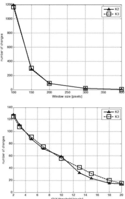
우선 윈도우의 크기의 영향을 알아보기 위해 RECC 윈도 우 크기를 100×100픽셀(100×100미터)에서 400×400픽셀까 지 변화시키며 변화지역을 탐지해 보았다. Fig. 3(a)의 그래프 에서 보인 것과 같이 윈도우 크기가 커질수록 변화지역으로
LiDAR system ALS50II
Acquisition date Feb. 17 2008 March 1,8,9,16 2008
April 14, 20 2008 Planned point density 5 points/m2
Image size 7,000×10,000 pixels Table 1. Specification of test LiDAR data
Satellite Kompsat-2 Kompsat-3
Acquisition
date 2010-02-07,
01:07(UTC) 2014-03-18, 04:29(UTC) Incidence/
Azimuth 5.8°/91.7° 25.9/145.0°
Original Ground Sampling Distance (line/
sample)
0.98/0.99 m 0.78/0.82 m
Orthorectified Ground Sampling Distance (line/
sample)
1.0/1.0 m 1.0/1.0 m
Image size
(line/sample) 7,000×10,000 pixels 7,000×10,000 pixels
Table 2. Specification of the orthorectified Kompsat data Fig. 2. LiDAR image and the orthorectified Kompsat images (a) LiDAR (b) Kompsat-2, (c) Kompsat-3
(b)
(c) (a)
263 도출되는 영역의 개수가 줄어들며, 윈도우가 200×200픽셀인
경우부터는 개수가 적절히 안정되는 것을 볼 수 있다. 윈도우 가 작을수록 세부적인 탐지를 볼 수 있으나 너무 작을 경우 윈 도우 내에 존재하는 의미 있는 에지 정보가 부족하여 유사성 분석이 힘들어질 수 있다. 따라서 200×200픽셀 정도의 윈도 우가 적절한 것으로 판단되었다.
두 번째로는 CV4의 영향을 알아보기 위해서 CV4 임계값을 2픽셀에서 20픽셀까지 변화시키며 변화지역을 탐지해 보았다.
이때는 윈도우의 크기를 앞서 언급한 200×200픽셀로 고정하 여, 영상 전역에 걸쳐 라이다 포인트가 불충분한 지역을 제외 한 총 211개의 영역에 대해 탐지가 수행되었다. 계산된 CV4가 임계값보다 큰 지역의 경우 에지값의 유사도의 정도가 적다고 인식되어 변화지역으로 분류되므로 임계값을 작게 설정할수 록 변화지역이 많다는 결과가 나오는 것을 Fig. 3(b)의 그래프 를 통해서도 확인할 수 있었다. CV4 임계값을 2픽셀로 설정한 경우 아리랑 2호의 경우 128개의 영역이 변화한 것으로 탐지 되었고 임계값을 20픽셀까지 높게 설정한 경우 14개의 지역만 이 변화한 것으로 분류되었다. 또한 아리랑 2호와 3호의 변화 지역의 개수가 거의 유사하게 탐지되는 것을 볼 수 있어, 변화 탐지에 일관성이 있음을 확인할 수 있었다.
다음으로는 변화 지역의 개수가 적절히 안정되는 200×200 픽셀로 윈도우 크기를 설정하고, 해당 윈도우 크기에서 변화 지역의 개수를 안정적으로 도출하기 위해 CV4를 3으로 선정 하여 이후 정확도 평가를 진행하였다. 변화 탐지 정확도 확인 을 위해 총 211개의 윈도우 영역내의 라이다와 위성영상을 절 취한 후 변화 탐지 결과를 모르는 작업자로 하여금 수작업으 로 변화 탐지 여부를 판독케 하였으며, 라이다-아리랑 2호 영 상 및 라이다-아리랑 3호 영상에 대해서 총 211개의 레퍼런스 데이터를 도출해 내었다. 이를 이용하여 본 논문에서 제시한 자동 탐지 기법 결과의 분류 행렬(confusion matrix)을 작성 하였으며 아래 Table 3과 Table 4에 제시하였다. 라이다-아리 랑 2호 영상의 변화 탐지 결과 전체 분류 정확도가 약 82.9%
이며, 사용자 및 제작자 정확도는 76~90%에 걸쳐 도출되었 다. 반면 라이다-아리랑 3호 영상의 경우 상대적으로 조금 낮 은 전체 정확도 79.1% 및 사용자 및 제작자 정확도 77~80.6%
를 보였다. 아리랑 3호 영상의 경우 입체 영상 취득을 위해 수직사진보다 상대적으로 높은 경사로 취득된 영상이기 때 문에 인공지형지물 등의 기복변위 등으로 기하학적인 차이가 많이 발생하여 변화 탐지 정확성의 저하가 나타낸 것으로 판 단된다.
Fig. 3. Number of detected changes as function of RECC window size and CV4 threshold
Kompsat-2 Reference
Changed Unchanged Sum Detected
Changed 85 26 111
Unchanged 10 90 100
Sum 95 116 211
Accuracy
Producer’s accuracy User’s accuracy Changed = 89.5% Changed = 76.6%
Unchanged = 77.6% Unchanged = 90.0%
Overall accuracy = 82.9 % Kappa coefficient = 0.66
Table 3. Accuracy of the change detection (LiDAR to Kompsat-2)
Kompsat-3 Reference
Changed Unchanged Sum Detected
Changed 87 21 108
Unchanged 23 80 103
Sum 110 101 211
Accuracy
Producer’s accuracy User’s accuracy Changed = 79.1% Changed = 80.6%
Unchanged = 79.2% Unchanged = 77.7%
Overall accuracy = 79.1%
Kappa coefficient = 0.58
Table 4. Accuracy of the change detection (LiDAR to Kompsat-3)
Journal of the Korean Society of Surveying, Geodesy, Photogrammetry and Cartography, Vol. 33, No. 4, 259-266, 2015
264
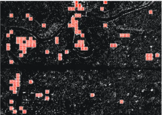
Fig. 4는 RECC를 활용한 변화 탐지 결과와 육안 판독을 통 해 취득한 레퍼런스를 아리랑 영상 위에 표시해본 그림이다.
빨간색 영역이 육안판독으로 변화지역으로 탐지된 지역이고 하얀색 박스 지역이 RECC를 통해 탐지된 변화 지역이다. 따 라서 빨간색 영역이지만 하얀 테두리가 없는 영역은 변화되었 으나 탐지가 되지 않은 지역이고, 점선 박스 지역은 변화지역 으로 탐지되었으나 육안 판독 상에서는 변화가 되지 않은 것
으로 나타난 지역이다. Fig. 4(a)의 아리랑 2호 영상 및 Fig.
4(b)의 아리랑 3호 영상 모두, 영상 좌측과 중앙 상단 쪽에 변 화 지역이 많이 형성되어 있음을 볼 수 있다. 참고로 라이다 데 이터의 중간 지역과 같이 점밀도가 현저히 떨어지는 지역은 변 화탐지가 시도 되지 않았다.
Fig. 4에 나타난 ID에 해당하는 변화 탐지 윈도우 영상의 예 를 아래 Table 5와 같이 제시하였다. 라이다 영상과 고해상도
Fig. 4. The detected region with the reference (the number within the box indicates the region ID) (a) LiDAR to Kompsat-2, (b) LiDAR to Kompsat-3
(a) (b)
Table 5. Sample patches of the change detection
ID LiDAR Kompsat-2 ID LiDAR Kompsat-3
6
Visual inspection : changed / RECC : changed 6
Visual inspection : changed / RECC : changed
78
Visual inspection : unchanged / RECC : changed 64
Visual inspection : unchanged / RECC : changed
88
Visual inspection : changed / RECC : changed
88
Visual inspection : changed / RECC : changed
98
Visual inspection : changed / RECC : changed
98
Visual inspection : changed / RECC : changed
146
Visual inspection : changed / RECC : unchanged 170
Visual inspection : changed / RECC : unchanged
265 위성영상간의 이질감으로 인해 판독이 어려운 경우가 있으나
기하학적으로 경계 정보가 명확히 차이가 날 경우 변화된 영 역으로 잘 탐지함을 알 수 있다.
3.3 분광정보 기반 변화탐지와의 비교
본 연구 방법의 비교를 위해 판별함수 (discriminant fun- ction) 기법을 적용하였다. 판별함수 기법은 해당 화소 주변 의 분광정보 분포를 이용하여 동일 위치의 두 시기의 변화가 능성 (확률)을 계산하는 방법으로서 단순한 정규 이미지 차 분법 (normalized image difference)보다 신뢰도가 높다. 판별 함수 기법은 변화 전, 후 영상에 대해 무감독분류를 실시하고 두 시기 영상간의 변화의 가능성을 계산하기 위해 판별함수 분석을 실시하여 결과 영상을 생성한다. 결과 영상은 0에서 1 사이의 값을 갖는 단일 밴드 (greyscale)영상이며, 0에 가까울 수록 변화의 가능성이 낮고 1에 가까울수록 변화의 가능성이 크다는 것을 의미한다.
실험에 사용된 라이다 영상 및 아리랑 영상 세트에 대해 판 별함수를 적용하여 0.95 이상 변화율이 존재하는 지역을 도 출하였고, 앞서 육안 판독으로 획득한 변화 지역과 함께 표 시하여 Fig. 5에 제시하였다. Fig. 5에서 하얀색으로 나타난 지역이 0.95이상의 확률로 변화지역으로 감지된 지역이다. 화 소값의 특성 자체가 크게 다른 이종 데이터의 특성상 판별함 수를 통해서도 유사성이 많이 발견되지 않아 변화 지역이 영 상 전역에 걸쳐 도출된 것으로 보인다. 또한 픽셀간의 연결성 을 통해 작은 픽셀 그룹을 제외하고 큰 변화 영역만을 필터링 해보았으나 큰 개선이 없음을 확인하였다. 따라서 본 연구에 서 제시한 에지 정보에 기반한 변화탐지의 효용성을 확인할 수 있었다.
4. 결 론
본 논문에서는 방사학적으로 이질성이 강한 이종 공간 영 상간의 변화 탐지를 위해 에지 유사성을 기반으로 한 변화 탐 지 기법을 제안하였다. RECC 기법은 윈도우 기반으로 단순하 고 빠른 연산이 가능할 뿐 아니라, 공간 영상간의 상호 좌표등 록이 정확하지 않더라도 적용이 가능하기 때문에 이종 데이터 의 변화 탐지에 제안되었다. 항공 라이다 데이터와 고해상도 위성영상인 아리랑 2호 및 3호 영상을 이용하여 실험을 수행 하고 윈도우 크기 및 RECC의 입력변수의 변화에 따른 변화 탐지 분석을 수행하였다. 또한 육안 판독으로 도출한 레퍼런 스 데이터에 비교하여 약 80%의 정확도의 변화 탐지율을 보 임을 확인하여 본 기법은 반자동 변화 탐지 기법 개발 시 효 용성이 높을 것으로 판단된다. 향후 변화 탐지된 영역 내에서 세부 변화영역을 도출하고 이를 정량화하는 연구가 필요하고 도시 내 식생 변화에 의한 영향에 대한 연구 또한 필요하다.
감사의 글
이 연구는 서울과학기술대학교 교내연구비의 지원으로 수 행되었습니다.
References
Chen, G., Hay, G.J., Carvalho, L.M.T., and Wulder, A. (2012), Object-based change detection, International Journal of Remote Sensing, Vol. 33, No. 14, pp. 4434-4457.
Chen, J., Gong, P., He, C., Pu, R., and Shi, P. (2003), Land- use/land-cover change detection using improved change- vector analysis, Photogrammetric Engineering & Remote Sensing, Vol. 69, No. 4, pp. 369-379.
Chen, X., Vierling, L., and Deering, D. (2005), A simple and effective radiometric correction method to improve landscape change detection across sensors and across time, Remote Sensing of Environment, Vol. 98, pp. 63-79.
Deng, J., Wang, K., Li, J., and Eng, Y. (2009), Urban land use change detection using multisensor satellite image, Pedosphere, Vol. 19, No. 1, pp. 96-103.
Fraser, C.S. and Hanley, H.B. (2005), Bias-compensated RPCs for sensor orientation of high-resolution satellite imagery, Photogrammetric Engineering & Remote Sensing, Vol. 71, No. 8, pp. 909-915.
Fig. 5. Change detection between LiDAR and Kompsat-2 based on the discriminant function (the boxes with ID
indicates the manually identified changed areas)
Journal of the Korean Society of Surveying, Geodesy, Photogrammetry and Cartography, Vol. 33, No. 4, 259-266, 2015
266
Lee, C.N. and Oh, J.H. (2014), LiDAR chip for automated geo-referencing of high-resolution satellite imagery, Journal of the Korean Society of Surveying Geodesy Photogrammetry and Cartography, Vol. 32, No. 4-1, pp.
319-326. (in Korean with English abstract)
Maas, J.F. (1999), Monitoring land-cover changes: a comparison of change detection techniques, International Journal of Remote Sensing, Vol. 20, No. 1, pp. 139-152.
Oh, J., Lee, C., Eo, Y., and Bethel, J. (2012), Automated georegistration of high-resolution satellite imagery using a RPC model with airborne lidar information, Photogrammetric Engineering & Remote Sensing, Vol. 78, No. 10, pp. 1045-1056.
Song, C., Woodcock, C.E., Steo, K.C., Lenney, M.P., and Macomber, S.A. (2001), Classification and change detection using landsat TM data: when and how to correct atmospheric effects, Remote Sensing of Environment, Vol.
75, pp. 230-244.
Zhang, H., Chen, J., and Mao, Z. (2009), An operational method to determine change threshold using change vector analysis, Proc. SPIE 7497, MIPPR 2009, SPIE, 30 October, Vol. 7497, pp. 749706~1-749706~8.