Comparison of Spatial Optimization Techniques for Solving Visibility Location Problem

(1)

가시권 문제를 위한 공간최적화 기법 비교 연구*

김영훈^1※¹⁾

Young-Hoon KIM^1※

요 약

지형분석에서 최대가시권역 확보 문제는 지리정보시스템 (GIS)의 가시권 분석에서 가장 널리 활 용되어 오고 있는 공간분석 방법이다. 그러나 한정된 자원과 제약 조건하에서 최대 가시권역을 확 보하는 지점을 탐색하는 공간 문제는 연산 과정이 복잡하고 이미 개발된 알고리즘의 경우, 본 연 구의 알고리즘과 차이가 있고 최대가시권역 문제 해결에 효과적으로 대처하지 못하고 있다. 그러 므로 본 논문에서는 최대 가시권역 문제를 GIS상의 공간 최적화 문제의 하나로 정의하고 이를 해 결하기 위하여 전통적인 시설물 입지 분석 알고리즘과 새로운 탐색 방법으로 일반적으로 비공간적 최적화 문제를 위해 개발, 제안되어 온 유전자 알고리즘과 시뮬레이트 어닐링 기법을 가시권 분석 문제에 적합하도록 개발하여 적용하였다. 이들 알고리즘의 적용 가능성과 성능 비교를 위해서 본 논문에서는 다양한 탐색 조건에 대한 각 알고리즘간의 가시권의 해 (visibility solution)를 비교하 고, 알고리즘의 탐색 안정성 (algorithmic consistency of solution values)을 통해서 최대가시권역 탐색에 적합한 기법들의 특징을 살펴보고자 하였다. 비교 결과, 유전자 알고리즘과 시뮬레이트 어 닐링 기법의 상대적 우수성과 GIS가시권 분석의 활용 가능성이 발견되었고, 향후 복잡하고 복합적 인 최대 가시권역 분석을 위해서 보다 향상된 탐색 알고리즘 개발의 필요성과 이를 통한 차세대 GIS가시권 공간분석 기법 개발을 제안하고자 하였다.

주요어 : 가시권 분석, 가시권역 문제, 최적화 알고리즘, 지리정보체계

ABSTRACT

Determining the best visibility positions on terrain surface has been one of the frequently used analytical issues in GIS visibility analysis and the search for a solution has been carried out effectively using spatial search techniques. However, the spatial search process provides operational and methodological challenges for finding computational algorithms suitable for solving the best visibility site problem. For this problem, current GIS visibility analysis has not 2006년 7월 20일 접수 Received on July 20, 2006 / 2006년 8월 31일 심사완료 Accepted on August 31, 2006

* 본 논문은 2005년도 한국교원대학교 교내 학술연구비지원에 의하여 연구되었음 (과제번호 RI20050130) 1 한국교원대학교 지리교육과, Department of Geography Education, Korea National University of Education

※ 연락저자 E-mail : [email protected]

(2)

been successful due to limited algorithmic structure and operational performance. To meet these challenges, this paper suggests four algorithms explored robust search techniques: an extensive iterative search technique; a conventional solution based on the Tornqvist algorithm; genetic algorithm; and simulated annealing technique. The solution performance of these algorithms is compared on a set of visibility location problems and the experiment results demonstrate the useful feasibility. Finally, this paper presents the potential applicability of the new spatial search techniques for GIS visibility analysis by which the new search algorithms are of particular useful for tackling extensive visibility optimization problems as the next GIS analysis tool.

KEYWORDS : Visibility Analysis, Visibility Location Problem, Spatial Optimization Algorithms, GIS

INTRODUCTION

Determining whether one point is visible from another on terrain surface and calculating the total visible area from one or more points are standard tools in Geographic Information Systems (GIS) and are often used in facility site selection applications including visibility location problem (Burrough and McDonnell, 1998). Visibility analysis has been also used to practical applications such as telecommunication relay tower location problem (De Floriani et al., 1994) and locating wind turbines (Kidner et al., 1999). With respect to search for optimal visibility location, the visibility problem is a spatial search problem that aims to search the maximum visible areas covered with the minimum number of viewpoints or observer sites on a digital terrain model (Kim et. al., 2004;

Kim, 2005). This problem takes two forms:

how much areas can be visible from n viewpoints, and what the minimum number of points is required to cover n percent of an area. The simple solution approach is to locate the points somewhere and then, calculate total visible areas within a GIS.

If the result is not satisfied, other points

are chosen by users or arbitrary manners and compare with the previous results.

This procedure is iterated until a satisfactory solution is met to the problem.

This simple method, however, suffers a serious drawback to search for optimal visibility locations on terrain surfaces. This location search problem dependents upon subjective choice of the user to choose points and it will cause numerous iterations and cannot guarantee an optimal solution if a larger digital terrain data is applied. For example, given a gridded Digital Elevation Model (DEM) data containing 1600 grid cells, every pixel can be a potential candidate for an optimal visibility site, which creates huge possible solutions. This means that the potential size of the search space becomes impracticable and that problem creates huge possible solutions. In theory, there are 2.9×1050 possible ways if ten viewpoints are searched for the best locations (e.g. P(10,1600) in combinatorial computation). If continuous space is applied for this problem, there are even more impossible solutions, because the possible viewpoint can be located at any DEM positions so that indefinite candidate numbers are generated. Hence, the problem

(3)

of locating a set of points that achieve maximum visibility is not simply to be solvable by a naive method or general iterative search techniques. To tackle this problem, therefore, the use of robust solution technique is required to meet these operational challenges in the visibility optimization problem.

Therefore, the objective of this paper is to discuss whether the use of optimization heuristics can lead to solutions to the visibility site selection problem, which are of good quality and computationally tractable. To obtain the research aim, in next section, this examines spatial optimization features of the visibility problem that enable existing optimization techniques to tackle successfully. In turn, this paper reports on a work that develops new solution algorithms by exploring existing optimization techniques. For new solution techniques, Genetic Algorithm (GA) and Simulated Annealing (SA) algorithm are modified to carry out the visibility site selection problem while a naive search algorithm using a set of random points and Tornqvist algorithm are used to compare their performances against the results of the new techniques. In next, experimental results of the optimization heuristics are discussed. The modification of their algorithmic structures that reflect the visibility location optimization nature would extend the application scopes of the optimization algorithms towards spatial optimization problems in GIS environment.

Finally, the functionality and success of the visibility optimization algorithms are discussed with the limitations and further research work issues.

VISIBILITY LOCATION PROBLEM

The works that has attracted a particular attention for visibility analysis problem as a spatial optimization problem are the development of visibility theories and algorithms, and the exploration of solution heuristics as an extensive facility location problem. The former approach includes introducing extensive visibility algorithms for computing various visibility information (De Floriani, 1994), graph theory for discrete visibility model (De Floriani, 1994), application of visibility graph to discrete visibility problems (Puppo and Marzano, 1997), and exploration of visibility graph methods for landscape evaluation (O'Sullivan, 2001). The latter approach includes optimal visibility site search problems such as the use of topographic features on terrain surface (Kim, et. al., 2004; Kim, 2005), discrete visibility network problem explored on TIN to link a set of communication stations with the use of visibility graph network algorithms (Lee, 1991; De Floriani, 1994) and the use of statistical sampling technique for finding optimal sites on terrain as a robust visibility solution algorithm (Franklin, 2000).

These theoretical achievements and application successes, however, left several unsolved tasks such as dealing with inordinate computing costs and exploiting robust solution heuristics for large visibility location problem.

The viewshed analysis quantified was only successful for a limited set of test locations or on simple gridded network model. Although the computing performance for large visibility data set has been identified in the literature, little work has been undertaken to explore possible solution algorithm on large visibility data sets.

(4)

PROBLEM REPRESENTATION

Since the visibility site selection aims to locate a set of points that maximise visibility, the problem is analogous with facility location planning which is to maximise customer accessibility. Thus the visibility site selection can consider a combinatorial problem for which heuristic solutions must be used. It is also almost analogous with facility location problem and the model formulation can be represented as followed.

Maximise Visibility, F(V) = ⁿ

φ

_ij

i m

j

vij

∑∑=1 =1

Subject to

0 ≤ ∑

= n

i

vij

1 ≤ n for j = 1, 2, 3, …, m

0 ≤ ∑

= m

j

vij

1 ≤ m for i = 1, 2, 3, … n

0 ≤ ∑∑

= = n

i m

j

vij

1 1 ≤ (n×m)

Where the visibility objective function represents F (V1,1; V2,2; V3,3; … Vn,m) in which Vi,j is the visibility Boolean of of ith visibility location on jth grid surface. The Vi,j

is true and counts 1 if i viewpoint can see the j surface cell, or false and counts 0 if not. Φij is to check overlapping visibility area of ith viewpoint such that if the surface cell is visible by previous site, the visibility count is not added even though it can be visible from the viewpoint. Thus, the cumulative intervisibility result is evaluated to meet the viewshed objective. n is the

number of viewpoints placed on the surface, m is the total number of cells of the surface.

For this analysis, a Digital Elevation Model (DEM) of the Cairngorm Mountain in Scotland from Digimap was used. The DEM data has a 50 meters spatial resolution and the elevation ranges from 263 meters to 1295 meters and contains 160000 grid cells which create a potentially large problem space for solving the visibility problem. In order to reduce the visibility computation, the DEM data was aggregated to 1 Kilometer resolution so that the data size is reduced to 400 grid cells. However, it is important to note that visibility problem is also applicable to 3 dimensional surfaces and artificial structures (i.e. buildings, houses, artefact features). However, as the research scope of this paper is focused on developing spatial optimization algorithms to visibility location problems and the comparison of the solution performances of the heuristics. Therefore, the issue for artificial structure remains further research agenda.

SPATIAL OPTIMIZATION HEURISTICS

1. Eight equi-spaced point method

The eight equi-spaced technique was originally built to determine new search neighbours within a SA algorithm used to solve a waste disposal site selection problem (Muttiah, et al., 1996). For efficient search way, their paper reported that the equi-space technique can contribute to achieve an impressive reduction of computing time by the circular search manner.

For the visibility problem, the search procedures can be used directly to find good

(5)

starting visibility locations on a DEM where each viewpoint has its own location information (e.g. coordinates) and elevation value. Using this data, the visibility quality (total viewsheds) of eight equi-spaced points in a circular neighbourhood is found.

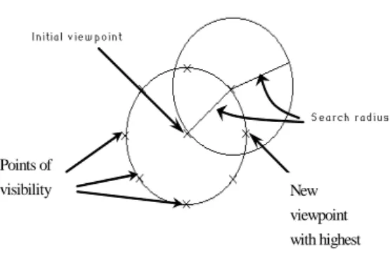
This neighbourhood search process is continued until no visibility improvement is displayed. For example, given a pixel randomly selected as an initial viewpoint, eight pixels around the point (e.g. North, West, East, South, North-West, North-East, South-West, South-East directed pixels) are selected for next candidate viewpoints to calculate its viewshed. Then, if one of the locations generates larger visibility solution, it replaces the initial location. This search process is continued until a termination condition (i.g. maximum search iteration) is met. Figure 1 illustrates the generation process of the eight equal spaced neighbourhood points for the visibility problem.

Initial v ie w p o int

Points of

visibility New

viewpoint with highest

S ea rch rad ius

Figure 1. Eight equi-circle technique for visibility site selection problem

The following psedo-code describes the visibility search procedures of the eight equi-spaced search technique.

Procedure eight equi-circle for the visibility site problem

begin

generate initial set of viewpoints compute visibility solution

bestViewPoint (Xi,Yi) ← initial viewpoints (Xi,Yi) while (until no visibility improvement)

while (until all viewpoints selected) do while (until all 8 direction selected) do compute visibility of the directed viewpoint if visibility is improved (better viewshed is found) then record the position information

(initial viewpoint (Xi,Yi) Neighbourhood (Xj,Yj) if any changes of locations found

then update the initial visibility location update visibility locations and visibility solutions, bestViewPoint (Xi,Yi) ← initial viewpoints (Xi,Yi) end

2. Tornqvist algorithm

In the late 1950s and early 1960s, Tornqvist, a Swedish geographer, developed a location optimization algorithm for solving facility location problems (Tornqvist et al., 1971). Although the Tornqvist algorithm was originally developed for solving multiple facility location analysis such as hospital location (Abler et al., 1968), the algorithm has been widely used for other optimal facility site problems such as urban facility planning (Hodgart, 1978), road network and service accessibility (Robertson, 1974;

Robertson, 1976) and recently transmit stations (Krzanowski, 1999). To be a robust location heuristic for the visibility problem, the algorithm employed a unique explorative search technique that examines its solution one step at a time along a west and east direction and a south and north direction until no further reduction in the objective function can be obtained. The following

(6)

pseudo-code describes the iteration search steps of the Tornqvist algorithm derived for the visibility problem.

Procedure Tornqvist algorithm for the visibility problem

begin

set control parameters (e.g. step sizes, decrease rate, minimum step length)

generate initial set of viewpoints compute visibility solution

bestViewPoint (Xi,Yi) ← initial viewpoints (Xi,Yi) while (until all viewpoint move) do

begin

move for a direction

compute a new visibility solution if the new solution not better if all direction tested break

else

change direction end

update visibility location

keep the best visibility locations, bestViewPoint (Xi,Yi)

end

3. Genetic algorithm

A genetic algorithm (GA) is a search algorithm that applies evolutionary rules and biological operators to solve complex optimization problems (Goldberg, 1989). New potential solutions are generated by the processes analogous to evolutionary biological mechanism. 'Good' new solutions are survived because they are better able to breed and replace each member of the old population by a newly bred individual. For solving the visibility problem, a potential solution to the problem is represented as a 'binary gene' - a fixed number of binary

bits. To develop evolution process, the GA requires a genetic plan, such as population size or offspring numbers, the number of generations, and the probabilistic rates of genetic operators such as crossover and mutation. Then the GA randomly selects an initial population representing binary bits to generate starting solution that converts numeric coordinates of visibility site pixels to a set of binary bits. The fitness of the current visibility solution (i.e. total visible cells) is then evaluated to determine whether this solution can be used for a new population by the selection rules in the GA process. In next, a new population sets are created from the selected old generation by applying the genetic operators. This evolutionary process is continued until a termination condition is met for which a fixed generation number is used in this paper. The following pseudo-codes present the visibility GA that reflects all evolution processes.

Procedure Visibility GA begin

set evolution parameters

(e.g. population size, Pc = 10, terminate condition, tmax = 100

Crossover rate = 0.95, mutation rate = 0.01) generate genetic populations, P1,2, … 10 /* Initialisation compute the visibility solution, F(vj) (j ← 1 to Pc)

/* Parent generation

for t ← 1 to tmax do // tmax is maximum generation number

select P(t) from P(t-1) apply fitness scaling

for j ← 1 to Npop do /* Npop Pc select two parent individuals from P(t) at

random

(using random probability weighted selection method)

(7)

apply crossover and mutation compute visibility, Fnew(vj) return P(t) ← Fnew(v)

update visibility solution among, Fold,new(v) /* Selection/replacement process

while j ← 1 to Npop do

find best new individual between F(C) and F(k) delete P(t) identical to P(t-1)

select worse individuals to die

(using random probability weighted selection method)

return create a new P(t+1) among P(t) and P(t-1)

return best visibility solution, F(vbest) and its visibility site information

end

4. Simulated annealing algorithm

Why SA algorithm is suitable for the visibility problem is that at first, maximum visibility sites generates multiple suboptima, which means that there may exist several different visibility locations representing same visibility on a DEM. Secondly, traditional hill climbing or random search methods (e.g.

Monte Carlo optimization search types) can get stuck in local suboptima since a move is only made when a better solution is found whilst simulated annealing technique can overcome the local optimum with robust probabilistic selection method, called the metropolic criterion (Kirkpatrick, et. al., 1983).

One solution for this drawback is to restart the search several times from different random starting solution and choose the best one. The 8 equi-circle and Tornqvist methods in this paper employ this approach.

Alternative, this paper switches to a superior optimization technique based on the traditional search method, but offers a robust a Monte Carlo optimization technique for the

visibility problem that exists many of multiple visibility suboptima in the solution process

For the visibility annealing process, the visibility SA employs a binary search concept that reduces temperature rate by fraction of acceptance moves and acceptance rate of the Metropolis criterion at each search step. This approach is useful to determine a sufficiently slow annealing sequence relevant to the visibility optimization problem available so that there is a good opportunity that the optimal visibility solution is found. Also, the advantage of this method is that the run length of each temperature and cooling schedule (temperature decrease) are easily determined and well planned for the optimization solution (see Liu et al., 1994 for more details).

procedure Visibility SA problem begin

input the annealing parameters, Td, At, Nc, nL, r calculate a current visibility solution, vs

compute initial temperature, Tempt0 = vs * 100 while Nc ← 1 to 5

Naccept , nL = 0 While nL ← 1 to 100

select a new viewpoints in neighbourhood generate a new solution, vq

compute visibility differences, d ( vq - vs )

if d > 0 or ( [0,1.0] exp( ) Temp0

rand > d

) then Naccept = Naccept + 1

vs ← vq

if vs is best visibility solution then keep vbest

retrun

calculate dt = nL N ^accept

if dt > nL then Nc = 0

(8)

0 50 100 150 200 250 300 350 400

2 3 4 5 6 7 8 9 10

Observers

Visible cell numbers

1st 100 times 2nd 100 times 3rd 100 times 4th 100 times 5th 100 times

100 150 200 250 300 350 400

2 3 4 5 6 7 8 9 10

Observers

a. 8 equi-circle method b. the Tornqvist algorithm

150 200 250 300 350 400

2 3 4 5 6 7 8 9 10

Observers

150 200 250 300 350 400

2 3 4 5 6 7 8 9 10

Observers

c. the visibility GA d. the visibility SA

Figure 2. Comparison of the best solution values on the randomised restarting solution configuration else Nc = Nc + 1

if dt > Td then Tempt = Temp / 2 else Tempt = Tempt*r

return best visibility solution, vbest end

RESULTS AND DISCUSSION

Traditionally optimization techniques are sensitive of starting solution in the initial stage, which means that a good starting solution set may guarantee better solution result for solving an optimization problem.

To test the sensitivity of starting solution, this paper uses two experimental procedures that reflect random selection and equivalent starting solution environment in their search solution process. As the first

procedure, 'a randomised' starting solution method is employed that in all search iteration, a unique set of starting solution is applied for the heuristics whilst as the second procedure, 'an identical' starting solution method is employed that a set of same starting solution is used. The purpose of this procedure is to enhance the solution performance comparison of the four algorithms by using the same restarting solution configuration in their search iterations.

Thus, the algorithms can start with the same restarting configuration to reduce the solution variation which occurs in the first procedure. In order to develop these two procedures, the number of viewpoints is

(9)

0 10 20 30 40 50 60 70 80

2 3 4 5 6 7 8 9 10

observer numbers

Standard deviation

50 100 150 200 250 300 350 400

Std. Dev.

Best value Average value Worst value

0 5 10 15 20 25

2 3 4 5 6 7 8 9 10

Standard deviation

100 150 200 250 300 350 400

Std. Dev.

0 2 4 6 8 10 12 14 16

2 3 4 5 6 7 8 9 10

Standard deviation

150 200 250 300 350 400

Std. Dev.

0 2 4 6 8 10 12

2 3 4 5 6 7 8 9 10

Standard deviation

150 200 250 300 350 400

Std. Dev.

c. the visibility GA d. the visibility SA Figure 3. Comparison of the solution values on the randomised restarting configuration

pre-defined to the limits of the viewpoint numbers, m (i.e. 1 ≤ m ≤ 10). In this experiment situation, the entire surface is not necessarily covered by the pre-specified viewpoints. The locations of the specified viewpoints are selected as a starting solution so that the visible regions from all viewpoints is maximised.

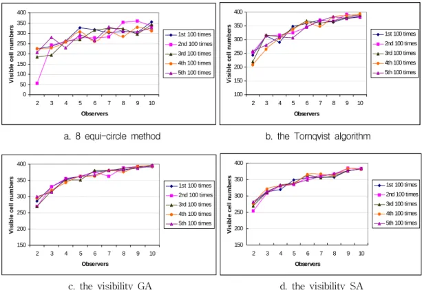
In the first procedure, the viewpoints are placed at random over a DEM grid surface and each run of the four algorithms constitutes several attempts at the placement of viewpoints. For this purpose, the four algorithms were run for 100 times with different starting viewpoint coordinates randomly generated in the iteration. The best solution result

(maximum visible cell numbers) out of those iterations is retained as a final optimal result. Figure 2 shows the solution values of the four algorithms, which elucidates the outperforming features of the new algorithms (GA and SA) in terms of solution quality (efficiency) and solution consistency. For all visibility problems (m

= 1, … ,10), the GA and SA methods outperform the traditional methods, especially for small visibility sets ( m = 2, 3, 4 cases). This figure also shows the solution stability of the GA and SA methods for various starting solution environments.

For the solution stability, Figure 3 shows the algorithmic consistency for the various

(10)

100 150 200 250 300 350 400

2 3 4 5 6 7 8 9 10

Observer numbers

100 150 200 250 300 350 400

2 3 4 5 6 7 8 9 10

Observer numbers

100 150 200 250 300 350 400

2 3 4 5 6 7 8 9 10

Observer numbers

100 150 200 250 300 350 400

2 3 4 5 6 7 8 9 10

Observer numbers

c. the visibility GA d. the visibility SA Figure 4. Comparison of the solution consistency on the same initial restarting configuration visibility problem cases of the four methods.

Regardless of the restart configuration condition, the genetic algorithm always outperforms the other methods, and the GA and the SA shows its algorithmic consistency over the two conventional methods by the standard deviation values.

These two results (Figure 2 and 3) show that even if a poor starting configuration (i.e.

remotely located candidate observer position) is given to the GA and SA algorithms, they can generate good solution results for the visibility site problem. In addition, these two modern heuristics are more independent on the starting solution in optimal solution search process.

For the second procedure that implements

same starting configuration, figures 4 and 5 present the comparison of the best solution values and the standard deviation values, respectively. For this experiment, 25 sets of the same initial viewpoints are prepared for each restarting configuration. For all given visibility sites, the genetic algorithm almost outperforms the other three algorithms in terms of the visibility solution. In particular, the maximum visible cell numbers are 397 for ten viewpoints case, which indicates that from the viewpoints almost the entire surface region can be seen. In this solution configuration, the 8 equi-circle method shows improvement for all most cases when compared with the result in Figure 2.

(11)

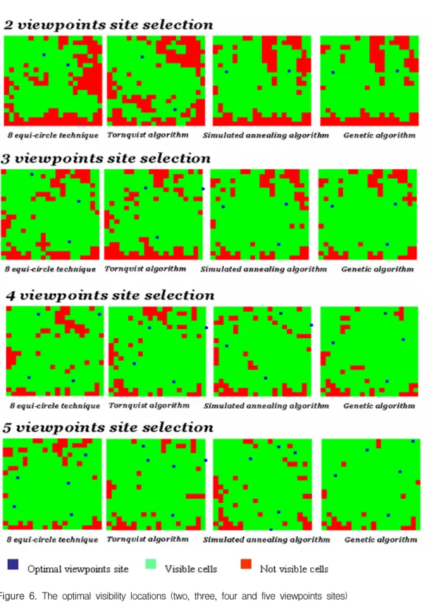
Figure 6. The optimal visibility locations (two, three, four and five viewpoints sites)

(12)

0 5 10 15 20 25 30 35 40 45

2 3 4 5 6 7 8 9 10

Standard deviation

100 150 200 250 300 350 400

Std. Dev.

Bes t value Average value Worst value

0 5 10 15 20 25 30 35

2 3 4 5 6 7 8 9 10

Standard deviation

100 150 200 250 300 350 400

Visible cell numbers Std. Dev.

0 2 4 6 8 10 12

2 3 4 5 6 7 8 9 10

Observer numbers

Standard deviation

100 150 200 250 300 350 400

Visible cell numbers Std. Dev.

Best value Average value Worst value

0 2 4 6 8 10 12 14

2 3 4 5 6 7 8 9 10

Standard deviation

100 150 200 250 300 350 400

Std. Dev.

c. the visibility GA d. the visibility SA Figure 5. Comparison of the solution values on the same initial restarting configuration

visibility sites (m cases)

2 3 4 5 6 7 8 9 10

8 equi-circle 37.13 39.59 23.58 25.65 21.30 18.12 25.01 16.17 16.23

Tornqvist 29.30 16.89 12.16 13.13 7.53 9.76 5.41 5.75 3.03

Genetic

alglorithm ^10.10 ^4.52 ^8.82 ^8.78 ^10.75 ^5.04 ^5.60 ^4.36 ^3.99

Simulated

Annealing ^8.25 ^11.88 ^6.54 ^5.22 ^4.36 ^4.43 ^3.68 ^3.48 ^2.93

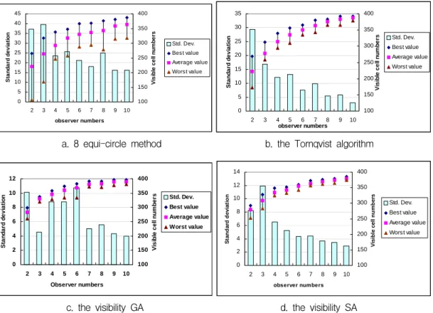
Table 1. The standard deviation values on the same initial restarting configuration The algorithmic consistency is clearly

identified in Figure 5 that shows the various solution set comparisons for the four algorithms. As with the results shown in the previous section, for all given visibility sites, the GA and the SA algorithms produce the most consistent solution performance relationship over the 8 equi-circle and

Tornqvist algorithms. Regardless of initial solution conditions, the GA and SA develop their search procedures using superior solution selection techniques such as evolutionary operators, crossover and mutation (genetic algorithm) and metropolis criterion (simulated annealing). The common feature of these two algorithms that shows

(13)

this superiority is a specified probabilistic rule to search for the best optimal solution so that the convergence ranges are reduced as the search iteration increases. Thus, whether good or poor candidates are assigned into initial starting procedure, the solution ability of the two intelligent algorithms converges at near global or global optimum because of their unique solution selection techniques. Therefore, the independence of the initial solutions and distinctive search manner provide the two intelligent algorithms with consistent solution generation for various optimization situations.

Table 1 shows the algorithmic consistency of each algorithm with the standard deviation values of the visibility solutions. At first it is recognised that the differences of the standard deviations decrease as the number of sites increases. This is because as the number of visibility sites increased, the search space to find the best optimal visibility position is reduced. It is clearly found in the comparison between the two viewpoints sites problem and the ten viewpoints site problem. Secondly, the consistency appears clearly up to five visibility sites. For example, the visibility solution of the SA method maintains a stable solution quality superior to all the others. As the experiments from two to five visibility sites allow larger search spaces than the tests from six to ten visibility sites, it can be inferred that given larger search space or problem sets to the GA and SA algorithms, their better solution performances that outperform the conventional algorithms can be confirmed.

For the optimal locations of the viewpoints, Figure 6 shows the best visibility sites of the

viewpoints of Figure 5. Whilst all algorithms present different visibility locations in each visibility problem, they present the influence of visibility location to visibility evaluation on the maps. Even though similar optimal visibility sites are generated for some problems (e.g. the GA and SA for two and three sites problems), the similarity of the visibility solution is not identical as much as the locations; 328 and 338 visible cells of the GA and the SA for three sites problem.

This comparison also asserts the important role of the use of robust solution algorithms for the visibility site selection problem.

With regard to computational performance, the four algorithms produce different aspects compared to the visibility solution. It has been found that the two conventional algorithms always take less CPU time than than the GA and SA algorithms. In general, for the visibility site problems, the 8 equi-circle technique run 10 times faster than the Tornqvist algorithm, 20 times faster than the GA and 40 times faster than the SA algorithm. Users may accept the inferior visibility solution of the eight equi-circle technique because of its faster computing time whilst some users prefer the best visibility solution which can guarantee the best visibility. Given extra computing times, the user should take into account additional work spending times to explore the suitable parameters for the problems. In general, the conventional algorithms require more extra works than the GA and SA because the GA and SA are more flexible to set up parameters than the conventional algorithms.

Therefore, for the computational performance, there exists a trade-off problem which the users should decide.

(14)

CONCLUSION

The paper raises several discussion points.

At first, the GA and SA algorithms have been shown to be largely independent of the starting values, which is a critical input in the conventional algorithms. The SA algorithm makes less stringent regularity assumptions regarding the objective function than do the conventional algorithms.

Exploring the whole search surface and attempting to optimise through both extensive uphill and downhill movements provide the SA algorithm with the superior algorithmic stability for the visibility optimization problems while the genetic algorithm produces an outstanding performance in generating better visibility solutions than the other three algorithms.

Secondly, like the previous algorithm benchmark tests, the conventional hill-climbing search approaches (8equi-circle and Tornqvist algorithms) have not outperformed the intelligent optimization techniques but for some visibility sites, the Tornqvist algorithm has generated a better solution than the SA. However, this has been at the expense of an unstable algorithmic performance and extra experiments to find adequate parameters. In addition, as shown in other location optimization problems, the visibility optimization process is also faced with the difficulty of the search process where the best local or global optimum is not always found from inside or around of neighbours containing good solution sets (local optimum). To tackle this problem, the GA and SA algorithms have applied their unique evolution rules and probabilistic selection method and they show the better

solution qualities and algorithmic stability.

Thirdly, in respect of algorithmic structure, it is possible to combine the features of the GA and the SA algorithm into a hybrid algorithm. This hybridisation approach can transfer the GA or SA to suit an optimal visibility site selection effectively and incorporate the positive features of the current algorithm in the GA or SA. A suitable hybrid algorithm may provide a better solution and computing performance.

However, there are no specific strategies to design a good hybrid algorithm. Therefore, the finding of a successful hybridization strategy for the visibility analysis should be the next work for this study.

In conclusion, as the algorithms have been applied to solve the visibility optimization problem, the application scopes of the visibility algorithms can be extended into various visibility analysis fields and the solution performances of the intelligent algorithms can be also compared with the conventional algorithms. Under the reasonable speedy computing environments it has been found that the GA presents the best solutions and the SA algorithm presents the most robust algorithmic consistency for various restarting solution conditions.

REFERENCES

Burrough, P. and C. McDonnel. 1998. Principles of Geographical Information Systems.

Oxford University Press, Oxford, UK. 333pp.

Floriani, L.D., P. Marzano and E. Puppo. 1994.

Line-of-sight communication on terrain models. International Journal of Geographical Information Systems 8(4): 329-342.

Goldberg, D.E. 1989. Genetic Algorithms in