Bridge Health Monitoring with Consideration of Environmental Effects

Bridge Health Monitoring with Consideration of Environmental Effects

Yuhee Kim*, Hyunsoo Kim*, Soobong Shin*^✝ and Jong-Chil Park**

Abstract Reliable response measurements are extremely important for proper bridge health monitoring but incomplete and unreliable data may be acquired due to sensor problems and environmental effects. In the case of a sensor malfunction, parts of the measured data can be missing so that the structural health condition cannot be monitored reliably. This means that the dynamic characteristics of natural frequencies can change as if the structure is damaged due to environmental effects, such as temperature variations. To overcome these problems, this paper proposes a systematic procedure of data analysis to recover missing data and eliminate the environmental effects from the measured data. It also proposes a health index calculated statistically using revised data to evaluate the health condition of a bridge. The proposed method was examined using numerically simulated data with a truss structure and then applied to a set of field data measured from a cable-stayed bridge.

Keywords: Bridge Health Monitoring, Data Analysis, Missing Data, Environmental Effects, Health Index

[Received: October 25, 2012, Revised: December 5, 2012, Accepted: December 10, 2012] *Department of Civil Engineering, Inha University, 100 Inharo, Nam-gu, Incheon 402-751, Korea, **Korea Expressway Co., Kyunggi-do, Korea ✝Corresponding Author: sbshin@inha.ac.kr

ⓒ 2012, Korean Society for Nondestructive Testing

1. Introduction

Large scale infrastructure, such as roads, bridges, dams and tunnels, require to secure structural integrity because they are frequently exposed to hazardous conditions. Since a struc- ture can face unexpectedly severe conditions due to overloaded vehicles, natural disasters, such as typhoons, and environmental actions, it is essen- tial to maintain the structural integrity by monitoring the health condition [1,23]. In partic- ular, it is critical to monitor in a systematic manner the health condition of special structures, such as long span bridges.

Structural health monitoring(SHM) for struc- tural systems has been studied since the 1970s but extensive studies of SHM of bridge structures began only in the early 2000s, as illustrated in Fig. 1 [10]. Fig. 1(a) shows the number of papers published annually in international journals by the end of 2010 searched using the keyword ‘SHM’ only, and Fig. 1(b) the number of reports obtained using

the keywords, ‘SHM’ and ‘bridge’, through the service of LANDSCOPE [10]. Fig. 2 also illustrates the number of papers published annually in international journals for research related to ‘temperature’ problems with the keywords (a) ‘temperature’ and ‘SHM’, (b)

‘temperature’, ‘SHM’ and ‘bridge’, and (c)

‘temperature’ and ‘bridge’. Research into temperature problems in bridge structures has a long history since the 1940s (Fig. 2(c)). On the other hand, research on SHM considering temperature effect has a relatively short history (Fig. 2(a)). In particular, the research on bridge structures started only recently, as shown in Fig.

2(b). Thus Figs. 1 and 2 highlight the need for more research related to SHM for bridge structures considering environmental effects.

The steps for SHM are normally divided as

follows: (1) processing and analyzing the

measured data, (2) diagnosing the structural

health condition, (3) locating structural damage,

and (4) assessing the severity of damage. In

some cases, steps (2) ~ (4) can be reduced to 1

(a) Searched with the keywords of ‘SHM’

(b) Searched with the keywords of ‘SHM’ & ‘bridge’

Fig. 1 Number of papers published in international journals related to ‘SHM’ [10]

(a) Searched with the keywords of ‘SHM’

(b) Searched with the keywords of ‘SHM’ & ‘bridge’

(c) Searched with the keywords of 'temperature' & 'bridge' Fig. 2 Number of papers published in international

journals related to ‘temperature’ [10]

Fig. 3 Schematic view of the current research scope

or 2 steps and then another step of determining the prognosis can be added. The current paper focuses only on steps (1) and (2); setting up the procedure for data analysis and defining a health index to judge any structural abnormality. Since many studies have evaluated data processing, this study presumes that the data provided from field measurements has already been treated by filtering out noise. Under this assumption, this paper narrows the scope down to (1) recovery of missing data, (2) consideration of environmental effects on the measured data, and (3) calculation of a health index to evaluate the global health condition of a particular structure. In each step, an effective method is selected from the methods available in the literature and modified for the current purpose. Fig. 3 shows a schematic diagram of the scope of current research.

A simulation study was carried out on a two-span truss structure to examine the proposed procedure of data analysis and the effectiveness of the health index. The measured data was simulated according to the temperature variations.

The method was then applied to field data measured from an actual cable-stayed bridge open to public transportation on a highway. This paper evaluates and discusses the results obtained.

2. Data Analysis Considering Environmental Effects

2.1 Recovery of Missing Data

Some parts of measured data can be missing

Fig. 4 Measured deformation with missing parts [18]

due to a malfunction of sensors or some other reason, as demonstrated in Fig. 4. In this case, it is essential to first recover the missing parts of the measured data to monitor the structural integrity more reliably.

Several methods have been introduced to estimate such missing data. Sohn [21] derived a linear regression model with the measured temperature variations and natural frequencies, and then applied this model to predict the natural frequencies for the next year using the measured temperature variations. Serker et al.

[20] also used a similar approach using a linear regression model but applied it to measured strain data rather than acceleration data. On the other hand, they also had to derive a regression model with the measured data of the previous year as baseline information. Peeters and Roeck [17] derived an ARX model using the measured temperature variations and natural frequencies up to four low modes, and applied that model to predict the natural frequencies of the next year with the measured temperature variations. Kullaa [8,9] proposed methods for recovering missing or incomplete data using the correlation in-between measured data. This method demonstrated the advantage of its possible applications to various types of measured data.

Nevertheless, it still required a set of baseline information to derive its model.

Another approach using a back-propagation neural network(NN) algorithm was proposed

[26]. Natural frequencies and mode shapes were used as the input neurons, whereas the target data corresponding to the input data were used as the output neurons. The error between the calculated output and target output values were back-propagated through the layers repeatedly to revise the weightings. Since the success of such a NN algorithm is dependent on the quality of training under a range of environments, it is essential to carry out an adequate amount of learning processes before applying the NN model to field data. Ko et al. [6] employed a similar approach for the Ting Kau Bridge in Hong Kong. They trained a NN model using the measured temperature variations and natural frequencies obtained for a one year period. Ni et al. [16] also employed a NN model for a bridge, measuring the same types of data, temperature variation and natural frequencies.

They used the data measured for 770 hours as the baseline information to train their NN model with all four layers including the input, output and hidden layers.

Since previous studies demonstrated that a bridge structure normally shows a good correlation between the natural frequencies and temperature variation, it is clear that a conspicuous pattern between them might be recognized easily by a NN approach. Therefore, this study employed the concept of a NN approach to recover missing data.

2.2 Elimination of Environmental Effects

The effects of environmental actions on the

structural dynamic behaviors have been studied

widely in SHM because structural dynamic

characteristics, such as natural frequencies and

mode shapes, are influenced more by environ-

mental conditions, such as temperature variation,

as shown in Fig. 2. Some studies on bridge

structures indicated that temperature variations

might be the most influential environmental

parameter [11,15,21,24]. A range of studies concluded that the health condition can be monitored more reliably using revised data by eliminating the environmental effects from the measured data [3,26].

A range of methods have been introduced in the literature to eliminate the environmental effects from the measured data. Conventional approaches include regression analysis [17], novelty detection [12], missing data analysis [8,9], singular value decomposition [19,22], and a support vector machine [15]. Another approach evaluating the environmental effects statistically with measured signals only without using an analytical model includes principal component analysis(PCA) [25], factor analysis [5,7] and neural network(NN) [6]. Since a signal-based approach is more feasible in field applications, this paper adopted the PCA method and modified it to the current research purpose by eliminating the environmental effects from the measured data.

The main idea of the PCA method is to reduce a matrix of natural frequencies,

, with n modes and N samples to a matrix,

, with only m principal components by multiplying a loading matrix

, as expressed in Eq. (1) [25].

X  T Y

(1)

where X is a linearly projected matrix onto a domain ℜ

from a domain ℜ

of

where

  

.

If m principal components can be selected by considering environmental effects on the natural frequencies, the matrix

can be considered to contain only the environmental aspects in the natural frequencies. The loading matrix

can be obtained by selecting m eigenvectors ordered by the larger values of a covariance matrix or by selecting m larger singular values. The current approach employed a singular value decomposition to calculate the

principal components using Eq. (2).

Y Y^T U



⁽²⁾

where

is an orthogonal matrix and  ^is

a diagonal matrix containing singular values.

The loading matrix

consists of the components from the 1

to the m

row vectors ordered by larger singular values.

Since the projected matrix

contains an environmental aspect only, the error information can be obtained by subtracting

from

. On the other hand, the domain size ℜ

of

is generally different from the domain size ℜ

of the original matrix

. Therefore, it is essential to back-project

to

in the original domain ℜ

using Eq. (3) and then to calculate the error by eliminating

from

, as expressed in Eq. (4).

Y_env T^TX  T^TT Y

(3)

Y  Y  Y_env

(4)

2.3 Calculation of the Health Index

The global structural health condition can be evaluated using the error matrix

of Eq. (4).

In the current approach, the structural health condition is evaluated by comparing the current condition to the baseline information of a presumably intact condition. Local damage detection and assessment are out of the scope of the current research because natural frequencies are used as the major measured information from a bridge.

As one of the useful health indices, the

Mahalanobis norm has been used in some cases

[3,25]. On the other hand, it has been observed

that this index frequently oscillates severely out

of the bounds, particularly when there is severe

noise in the measured data. Therefore, this study

proposes a modified distance MD on the log

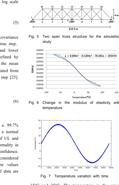
Fig. 5 Two span truss structure for the simulation study

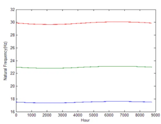
Fig. 6 Change in the modulus of elasticity with temperature

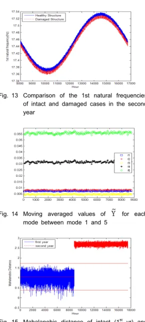
Fig. 7 Temperature variation with time

scale defined by Eq. (5) by applying a log scale to the original formulation.

(5)

where



is the covariance matrix of the matrix

and k is the time step.

The center line CL, the upper and lower limit lines of UL and LL, can be defined by Eq. (6) using the statistical values of the mean



 and standard deviation

calculated from the Mahalanobis distances at each time step [25].













(6)

If

= 3 is used in Eq. (6), a 99.7%

confidence level can be guaranteed in a normal distribution. Therefore, the limit lines of UL and LL can be used to determine any abnormality in the structural integrity with 99.7% confidence.

In other words, the structure can be considered to be in a healthy condition if the values calculated using a new set of measured data are within these limit boundaries.

3. Examination through Simulation Studies

3.1 Analytical Model for the Simulation Study

To examine the proposed procedure of data analysis and the health index of eqns. (5) and (6), a simulation study was carried out with a two-span truss structure, as shown in Fig. 5.

The area of each member was assumed to be 0.0025 m

and the mass density was 7,850 kg/m

. For the simulation study, the modulus of elasticity was assumed to vary with temperature, as shown in Fig. 6 [2]. Fig. 7 shows the annual variation of the daily mean temperature between

-15°C and 35°C. The temperature in the upper and lower chord members was simulated to be 5°C higher and lower, respectively, than that of the diagonal and vertical members. To simulate the measured temperature, a 1% random varia- tion in the modulus of elasticity was added arbitrarily to each member.

3.2 Simulation of Measured Data

Based on the information in Figs. 6 and 7,

the natural frequencies up to ten low modes

were calculated. Fig. 8 presents the variations of

the first three with time for one year. All 8,760

sampling data points for each mode were

Fig. 8 Change in natural frequencies with time

Fig. 9 Variation of the first natural frequency with time

(a) Whole range of the second year

(b) Hour: 10,801~11,100 (c) Hour: 15,301~15,600 Fig. 10 Prediction of the first natural frequencies in

the second year

obtained by calculating the natural frequencies once an hour for one year.

A NN model was defined using the measured natural frequencies of ten modes and the simulated temperature variation. The temperature variation of each member in time was considered as input values. The corre- sponding natural frequencies were the output values in the NN model. The number of neurons in the hidden layers was selected to minimize the estimation error. The tangent sigmoid function and linear function were used as transfer functions in the model.

The NN model was trained by the data for the first year and then used to predict the natural frequencies of the second year at various temperatures, as shown in Fig. 9 for the first natural frequency. In this paper, a NN model was defined for each mode separately. For the current simulation study, 35 neurons in one input layer, 40-60-20 neurons in the hidden layers, and 1 neuron in the output layer were selected.

Fig. 10(a) compares the simulated real data and the data of the first natural frequencies in the second year estimated from the trained NN model. Figs. 10(b) and 10(c) compare those two data regions in detail around the minimum and maximum values of the first natural frequencies inside the circles drawn in Fig. 10(a). Although those two regions had relatively higher error in the estimated results, the model trained with the first year data predicted the variation of the first natural frequencies quite reasonably.

3.3 Elimination of Environmental Effects

As shown in Fig. 10, the first natural

frequency varied with temperature and time. The

PCA method was applied to eliminate such

environmental action on the measured data. The

singular values of the measured data were

calculated (Fig. 11). Since ten low modes were

Fig. 13 Comparison of the 1st natural frequencies of intact and damaged cases in the second year

Fig. 14 Moving averaged values of Y for each mode between mode 1 and 5

Fig. 15 Mahalanobis distance of intact (1^st yr) and damaged structure (2^nd yr)

Fig. 11 Computed singular values for PCA

Fig. 12 Computed health index with a NN model trained with the first year data

measured from the simulated truss structure, the dimension n for the original modal information matrix

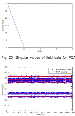
equaled 10. On the other hand, because only one singular value was clearly higher than the others, the dimension m for the projected domain of

equaled 1. In other words, temperature is the only influential environmental factor that should be eliminated from the data.

3.4 Calculation of Health Index

The log-scaled Mahalanobis distance was calculated using Eq. (5), and the CL, UL, and LL lines are drawn by Eq. (6) in Fig. 12. In Fig. 12, the first year data was used to train the NN model and to estimate the second year data.

The trained model could predict a healthy condition in the entire range of interest with some minor outliers below the lower limit line LL.

To confirm the utility of the health index, a damage case was simulated with reduced axial stiffness of the member in the upper chord

between nodes 14 and 15 in Fig. 5. For the simulation study, a 2% decrease in axial stiffness was assumed. Fig. 13 compares the change in the first natural frequencies of the intact and damaged cases in the second year.

The first natural frequencies of the damaged cases were slightly lower than those of the intact cases. The moving averages of the error

Y

of Eq. (4) are drawn in Fig. 14 for each

mode between modes 1 and 5. The figure shows

that the error due to damage is larger for a

0 500 1000 1500 2000 2500 0.2

0.21 0.22 0.23 0.24 0.25 0.26 0.27 0.28 0.29

Time(day)

F1(Hz)

0 500 1000 1500 2000 2500

0.27 0.28 0.29 0.3 0.31 0.32 0.33 0.34 0.35 0.36 0.37

Time(day)

F2(Hz)

(a) 1st natural frequency (b) 2nd natural frequency

0 500 1000 1500 2000 2500

0.48 0.49 0.5 0.51 0.52 0.53 0.54 0.55 0.56 0.57 0.58

Time(day)

F3(Hz)

(c) 3rd natural frequency (d) 4th natural frequency

0 500 1000 1500 2000 2500

0.58 0.59 0.6 0.61 0.62 0.63 0.64 0.65 0.66 0.67 0.68

Time(day)

F5(Hz)

(e) 5th natural frequency

Fig. 18 Variation of natural frequencies measured from a cable-stayed bridge for six years Fig. 16 View of the test bridge

□ accelerometer Fig. 17 Sensor layout for the maintenance of the

bridge

higher mode in general, even if all the error values are quite small.

Using the computed error

after elimi- nating the temperature effect, the Mahalanobis distances of Eq. (5) were calculated for the damaged case with the data of the second year and then compared with those of the first year (Fig. 15). The figure confirms that the health index used in the present study could clearly identify the health condition, even when only one truss member was damaged by a 2%

decrease in axial stiffness.

4. Application to Field Data

The field data measured from a cable-stayed bridge shown in Fig. 16 were used to confirm the usefulness of the proposed approach. The bridge is located in a highway crossing a sea channel. The total length of the cable-stayed bridge part is 990 m (60+200+470+200+60 m).

Various types of sensors were installed to measure the bridge behavior and environmental actions, as shown in Fig. 17. Among them, the

data measured from the temperature sensors and accelerometers were used in the present study.

4.1 Data Processing of the Measured Data

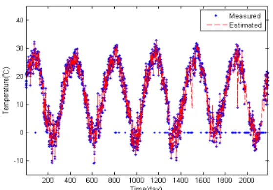
The natural frequencies measured from a cable-stayed bridge for six years, as shown in Fig. 18, were used to confirm the effectiveness of the proposed procedure. Fig. 19 shows the temperature variation between -10°C and 35°C measured from one of the six temperature sensors installed in the bridge during the same period. All the data was provided by the authority in charge of maintaining the bridge.

Each data point of natural frequency and

temperature was obtained by averaging one hour

of data measured every 10 minutes. The data

shown in Figs. 18 and 19 was drawn after

erasing some outlier data far from the general

trend. Since the measurement system was

installed more than 10 years earlier, the sampl-

ing rate was not detailed enough to give a

Fig. 19 Temperature variation during the measuring period

-15 -10 -5 0 5 10 15 20 25 30

0.254 0.256 0.258 0.26 0.262 0.264 0.266 0.268 0.27 0.272

TemTeTaTTTe(℃)

F1(Hz)

Fig. 20 Correlation between the first natural fre- quency and temperature (R=0.714)

Fig. 21 Comparison of the measured and estimated temperature variation by a NN model

Fig. 22 Comparison of measured and estimated natural frequencies by a NN model

satisfactory outcome. Nevertheless, the variations of the first, third, and fifth natural frequencies in Fig. 18 showed sinusoidal patterns that might correlate with the temperature variation in Fig.

19. On the other hand, it was difficult to observe any vivid pattern in the measured even modes, possibly due to the triggering process on the raw data carried out by the maintenance authority. Fig. 20 shows the correlation between the first natural frequency and temperature; their computed correlation factor was 0.714. This suggests that the two data measurements correlated well but not linearly.

4.2 Data Analysis and Prediction

Before developing a NN model between the measured temperatures and natural frequencies, the missing parts in the temperature variation

were first estimated by applying another NN model. Fig. 21 shows the estimated temperature variation with the filled missing parts by the NN model compared to the original measured data in Fig. 19.

A NN model was then trained for each

mode using the first two-year measured data of

natural frequencies and temperature. Each NN

model was defined with five layers including 1

input layer with 7 neurons, three hidden layers

with 25-40-7 neurons, and 1 output layer with 1

neuron. The input data for the NN model of the

temperature variations comprised the temper-

atures measured at the lower parts of the

girders, crossbeams and the upper parts of the

girders in the bridge. Fig. 22 compares the

measured and estimated natural frequencies by

the trained NN model for six years. The overall

variations show a reasonalble match, as demon-

Fig. 23 Singular values of field data for PCA

Fig. 24 Comparison of estimated natural frequencies Y by the NN model and its Y_{e n v}

0 200 400 600 800 1000 1200 1400 1600 1800 2000 -5

-4 -3 -2 -1 0 1 2 3 4

5 PCA Model : SVD

Time(day)

Mahalanobis DisTance

baseline moniToTed

(a) Mahalanobis distance defined by Eq. (5)

0 200 400 600 800 1000 1200 1400 1600 1800 2000 -1

0 1 2 3 4 5 6 7

8 PCA Model : SVD

Time(day)

Mahalanobis DisTance

baseline moniToTed

(b) Mahalanobis distance without log scale Fig. 25 Heath index of field data

strated in the figure. The missing data in the initial parts of the figures in Fig. 18 were recovered in Fig. 22 by applying the NN models.

4.3 Elimination of the Environmental Effect

Before calculating the health index, the environmental effects on the measured data should be eliminated. Fig. 23 shows the calculated singular values of the measured data, demonstrating that temperature is the only environmental factor affecting the vibrational aspects of the cable-stayed bridge.

Fig. 24 compares the estimated natural frequencies

using the NN model estimated in Fig. 22 along with its environmentally influ- enced data

by Eq. (3). The figure shows that the environmentally influenced data

varies along the estimated data

with narrower bands.

4.4 Calculation of the Health Index

The health indices of the Mahalanobis

distance defined by Eq. (5) were calculated for

six years using all the revised data, and are

drawn in Fig. 25(a). Fig. 25(b) also shows the

health index of the Mahalanobis distance

without a log scale for comparison. As demon-

strated in Figs. 21 and 22, the first two-year

data was used to train the NN models and the

next four-year data was predicted using the

defined model. Fig. 25 shows that some of the

peaks of the calculated health index around the

same season in a year were out of the lower

limit line. On the other hand, the overall

computed health indices were within the limit

boundaries. Compared to the health indices

calculated using Eq. (5), the health indices

without using the log scale of eqn. (5) showed

more vivid violations of the limit boundaries, as

shown in Fig. 25(b). Nevertheless, the health

condition of the bridge could be retained without serious changes or damage because the patterns of the health index for the test period were similar.

5. Conclusions

This paper suggested a systematic procedure for data analysis for reliable structural health monitoring by recovering the missing data and by eliminating the environmental effects in the measured data. A health index of the modified Mahalanobis distance was proposed to evaluate the structural health condition. Examination and verification through simulation studies and field applications demonstrated the usefulness and efficiency of the suggested procedure and proposed health index.

The use of PCA to simulated and field measured data confirmed that temperature variations was the most critical environmental factor affecting the dynamic characteristics of a bridge, even though the percentage variations of natural frequencies were relatively small, as revealed by Fig. 18. Since the change in natural frequencies showed a good correlation with the annual variation of temperature, the use of a Neural Network model in estimating the natural frequencies was found to be a successful choice and could provide reliable results.

The use of the Mahalanobis distance for a health index demonstrated a reliable prediction of bridge health conditions. The proposed log scaled formulation evaluated the health condition better than the original one. On the other hand, some distances calculated by the equation were out of the limit boundaries in both the simulated case and application to an actual cable-stayed bridge. Such an evaluation error by the Mahalanobis distance could be attributed to measurement noise or the poor quality of the measured information.

Since any damage can be identified as a continuous deviation from the intact case using the Mahalanobis distance, the proposed method could be applied reliably to structural health monitoring of a bridge based on the measured natural frequencies. Nevertheless, since the change in the natural frequencies may not reliably predict all structural abnormalities, it will be important to develop an advanced health index unifying all types of measured data concurrently in the future.

Acknowledgements

This study was supported by a grant of KICTEP 08-E01 from the Super Long Bridge R&D Center and Inha University.

References

[1] E. Aktan, F. N. Catbas, K. A. Grimmelsman and M. Pervizpour, "Development of a model health monitoring guide for major bridges," Drexel Intelligent Infrastructure and Transportation Safety Institute, pp. 183-230 (2003)

[2] ASME, Power Piping, ASME, B31.1 (1995) [3] A. Bellino, A. Fasana, L. Garibaldi and S.

Marchesiello, "PCA-based detection of damage in time-varying systems," Mechan- ical Systems and Signal Processing, Vol.

24, pp. 2250-2260 (2010)

[4] H. Cho, Y. Choi, S. Lee and K. Lee,

"Structural damage assessment based on model updating and neural networks,"

Structure Maintenance and Inspection, Vol.

7-4, pp. 121-128 (2003)

[5] A. Deraemaeker, E. Reynders, G. De. Roeck and J. Kullaa, "Vibration-based structural health monitoring using output-only measure- ments under changing environment,"

Mechanical Systems and Signal Processing,

Vol. 22, pp. 34-56 (2008)

[6] J. M. Ko, K. K. Chak, J. Y. Wang, Y. Q.

Ni and T.H.T. Chan, "Formulation of an uncertainty model relating modal parameters and environmental factors by using long-term monitoring data," Proceedings Smart Structures and Materials : Smart Systems and Nondestructive Evaluation for Civil Infrastructures 5057, 298-307 (2003) [7] J. Kullaa, "Damage detection the Z24

bridge using control charts," Mechanical Systems and Signal Processing, Vol. 17(1), pp. 163-170 (2003)

[8] J. Kullaa, "Damage detection under a varying environment using the missing data concept," Proceedings of the 5th International Workshop on Structural Health Monitoring, Stanford, CA.

September 12-14, Stanford University, DEStech Publications, pp. 565-573 (2005) [9] J. Kullaa, "Eliminating environmental or

operational influences in structural health monitoring using the missing data analysis,”

Journal of Intelligent Material Systems and Structures, Vol. 20, pp. 1381-1390 (2009) [10] LANDSCOPE, http://www.landmark.re.kr.

[11] H. Li, S. Li, J. Ou and H. Li, "Modal identification of bridges under varying environmental conditions: Temperature and wind effects," Structural Control and Health Monitoring, Wiley InterScience (2009)

[12] G. Manson, S. G. Pierce and K. Worden,

"On the long-term stability of normal condition for damage detection in a composite panel," Key Engineering Materials, Vol. 204-205, pp. 359-370 (2001)

[13] D. C. Montgomery, "Statistical Quality Control," WILEY (2009)

[14] M. Mehrjoo, N. Khaji, H. Moharrami and A. Bahreininejad, "Damage detection of truss bridge joints using artificial neural networks," Expert Systems with Applica-

tions, Vol. 35, pp. 1121-1131 (2008)

[15] Y. Q. Ni, H. F. Zhou and J. M. Ko,

"Correlating modal properties with temperature using long-term monitoring data and support vector machine tech- nique," Engineering Structures, Vol. 27, pp. 1762-1773 (2005)

[16] Y. Q. Ni, H. F. Zhou and J. M. Ko,

"Generalization capability of neural net- work models for temperature-frequency correlation using monitoring data," Journal of Structural Engineering, Vol. 135(10), pp. 1290-1300 (2009)

[17] B. Peeters and G. De Roeck, "One year monitoring of the Z24 bridge: Environ- mental influences versus damage effects,"

In Proc. IMAC-XVIII, San Antonio, TX, pp. 1570-1576 (2000)

[18] D. Posenato, P. Kripakaran, D. Inaudi and Ian F. C. Smith, "Methodologies for model-free data interpretation of civil engineering structures," Computers and Structures, Vol. 88, pp. 467-482 (2010) [19] R. Ruotolo. "Using SVD to detect damage

in structures with different operational condition," Journal of Sound and Vibration, Vol. 2206(3), pp. 425-439 (1999)

[20] N. H. M. K. Serker, Z. S. Wu and S. Z.

Li, "A Nonphysics-based approach for vibration-based structural health monitoring under changing environmental conditions,"

Structural Health Monitoring, Vol. 9(2), pp. 145-158 (2009)

[21] H. Sohn, "Effects of environmental and operational variability on structural health monitoring," Special Issue of Philosophical Transactions of the Royal Society, Structural Health Monitoring, Vol. 365, pp. 539-560 (2007)

[22] S. Vanlanduit, E. Parloo, B. Guillaume, P.

Cauberghe and P. Verboven, "A robust

singular value decomposition for damage

detection under changing operating condi-

tions and structural uncertainties," Journal of Sound and Vibration, Vol. 284, pp.

1033-1050 (2005)

[23] H. Wenzel, "Health Monitoring of Bridges,"

WILEY, pp. 1-17 (2009)

[24] Z. D. Xu and Z. S. Wu, "Simulation of the efect of temperature variation on damage detection in a long-span cable- tayed bridge," Structural Health Monitoring, Vol. 6, pp. 177-189 (2007)

[25] A. M. Yan, G. Kerschen, P. De Boe and J.-C. Golinval, "Structural damage diagnosis under varying environmental conditions - part I: A nonlinear analysis," Mechanical

Systems and Signal Processing, Vol. 19(4), pp. 847-864 (2005)

[26] H. F. Zhou, Y. Q. Ni and J. M. Ko,

"Constructing input to neural networks for modeling temperature-cause modal variability:

Mean temperatures, effective temperatures, and principal components of temperatures,"

Engineering Structures, Vol. 32, pp.

1747-1759 (2010)

[27] Y. Zhu, Y. Fu, W. Chen and S. Huang,

"Online deflection monitoring system for

Dafosi cable-stayed bridge," Journal of

Intelligent Material Systems and Structures,

Vol. 17, pp. 701-707 (2006)