?
Estimating Housing Prices through a Spatial GAMLSS Modeling Approach
Changro Lee* · Keyho Park**
공간 GAMLSS 모형을 활용한 주택가격 추정
이창로*·박기호**
Abstract : Estimation of housing prices is of great importance in various sectors, including property tax assess- ment and collateral valuation. The multi-household house (MHH) is an emerging property type for the appli- cation of the automated valuation method in South Korea. Thus we choose Seoul, the capital of South Korea, as our study area, and apply the hedonic price model to MHH, a common tool in property valuation. We suggest an alternative approach to estimate housing prices – generalized additive models for location, scale, and shape (GAMLSS) – in order to overcome the limitations inherent in the traditional hedonic price model, those limitations being: lack of theoretical background for a functional form, assumption of a linear relationship between the explanatory and response variables, and little account of spatial autocorrelation in model building.
We employ the GAMLSS with the spatial autocorrelation of the data being taken into account. We show that a non-normal distribution could give a better fit for house prices and illustrate nonlinear effects of the explana- tory variables, as well as the spatial effect of house locations on the price of MHH. We hope that the spatial GAMLSS modeling approach in this study will lead to better property tax assessment and collateral valuation.
Key Words : Housing prices, Multi-household house, GAMLSS, Spatial autocorrelation, Non-normal distri- bution, Nonlinear effects
요약 :과세평가, 담보평가 등 주택가격의 추정은 사회 여러 분야에서 중요한 의미를 갖는다. 아파트에 비해 상품
표준화 정도가 낮은 다세대주택의 경우 최근 자동평가모형의 적용 대상으로 부상하고 있다. 이러한 추세를 따라 주택가격 추정에 광범위하게 사용되는 헤도닉 모형을 적용하여 서울 소재 다세대주택의 가격을 추정하였다. 함수 형태의 이론적 근거 부재, 설명변수와 종속변수 관계의 선형성 가정, 공간적 자기상관성의 미고려 등 전통적 헤도 닉 모형이 갖는 한계를 극복하기 위해 본 연구에서는 공간 GAMLSS 모형을 제안하였다. 본 연구를 통해 주택가 격은 정규분포 이외의 분포를 가정하는 것이 보다 적절할 수 있고, 설명변수와 종속변수는 비선형 관계의 형태로 설계함이 타당하며, 마지막으로 주택의 지리적 위치에 따른 공간적 자기상관성 고려가 필수적임을 보였다. 공간 GAMLSS 모형 활용을 통해 과세평가나 담보평가에 있어 주택가격 추정의 정확성이 제고되기를 기대한다.
주요어 :주택가격, 다세대주택, GAMLSS, 공간적 자기상관성, 비정규분포, 비선형 효과
* Associate Research Fellow, Korea Institute of Local Finance, Researcher, Institute for Korean Regional Studies, [email protected]
** Professor, Department of Geography, Seoul National University, Researcher, Institute for Korean Regional Studies, [email protected]
1. Introduction
A residential building built for sale in units is generally referred to as ‘a multi-unit house’ in South Korea. The multi-unit house has several unique characteristics, such as the option of co-owning a site and forming a residen- tial community composed of inhabitants in the build- ing. The housing type obverse of the multi-unit house is the detached house, which is generally composed of one building and its corresponding site. The multi-unit house has enjoyed great popularity in South Korea in the past due to the scarcity of urban land available for buildings, and has taken a firm position as a representative hous- ing type in urban areas. The multi-unit house comprises an apartment and a multi-household house (hereafter, MHH). According to the Building Act in South Korea, if the floor area of the multi-unit house is over 660m2, then it is classified as an apartment; otherwise it falls under the category of MHH.
The valuation of housing is of great importance for both public and private sectors. Accurate assessment of properties is key in enhancing the taxation equity, and reliable estimation of housing collateral by financial in- stitutions plays a core role in keeping the collateral loans undoubtful. Since the apartment is the most standard- ized property type, it is relatively easy to apply an auto- mated valuation method and obtain a reliable estimate of the apartment market value. In contrast, the detached houses vary in terms of location, site characteristics, construction workmanship, etc. Thus, their valuations remain a realm for single-property appraisal, which is usually conducted by a licensed expert, and thus it would be premature to apply the automated valuation method.
MHH is situated between the apartment and the de- tached house in terms of applicability of a quantitative valuation technique, since it is a standardized property in part, but also shows unique characters such as location.
From the perspective of financial banks, they tend to
invest as little resource as possible to estimate the market value of MHH, since they think it is easy to evaluate the price of MHH. However, MHH is not the perfectly standardized property product, and has considerable risk that its estimated price deviates from its market value severely. Recently, methods such as the hedonic price model have slowly begun to apply to them in the South Korean real estate market. Therefore, the application of the automated valuation method to MHH is of great is- sue in valuation practices. We decide to choose MHH as a target property for applying the hedonic price model in this context.
The hedonic price model is generally used in property valuation, and is usually fitted by using regression analy- sis. Property price is broken down into its constituents such as land area, building area, presence of elevators, and others under the hedonic price model framework, and it produces estimates of the contributing value of each constituent, ultimately providing the whole value of the property by summing up each contributing value.
Although the hedonic price model is the most commonly used method in a quantitative property valuation, it has its own limitations and criticisms. The oldest and most severe criticism is that the appropriate functional form cannot be guided on theoretical grounds (Halvorsen and Pollakowski, 1981). In practice, the Gaussian distribu- tion is commonly assumed for the response variable, and a linear relationship between the explanatory and response variables is implicitly presumed in specifying the hedonic price model, leading to inefficiency and inac- curacy in price estimation.
We explore various functional forms for the response variable and try to specify an optimal form for the he- donic model. In addition, we step from the practice of as- suming a linear relationship between the explanatory and response variables, and instead try to capture the non- linear relationship between variables in the model speci- fication. In order to achieve these goals, we estimate the price of MHH under the framework of generalized addi-
tive models for location, scale, and shape (GAMLSS).
Since the hedonic price model has been sophisticated in economics since its proposal, the spatial component in model specification often went unnoticed in many previ- ous studies. However, it is well known that house prices are not distributed independently over space, but rather tend to show similar values in neighboring areas, which is often referred to as spatial autocorrelation (Basu &
Thibodeau, 1998; Tu et al., 2007). It indicates that even identical houses can be sold for vastly different prices de- pending on location, and thus the house price cannot be estimated reliably without careful consideration of house locations. It is the first law in property valuation, though it is frequently ignored when modelling house prices. We try to incorporate the spatial effects into the GAMLSS model specification in the study.
This study is organized as follows. The second section reviews the GAMLSS and relevant literatures, and the third section explains the data used and model specifica- tion. Model calibration and main results are provided in the fourth section, and finally, we present a discussion on the results and our conclusions.
2. Literature review
Literary volumes on the hedonic price model are vast in number, ranging from the seminal paper of Rosen (1974) to more recent studies (Mei et al., 2018; Michelson and Tully, 2018), but most of them bear the limitations given above: the conventional assumption of the Gauss- ian distribution for property price without the due atten- tion to the functional form, the presumption of linear relationships between the explanatory variables and property price, and the absence of explicit accounts of the spatial effects on the property price.
GAMLSS could be a suitable tool to overcome these traditional limits inherent in the hedonic price model.
GAMLSS were developed by Rigby and Stasinopoulos (2005) to deal with non-normally distributed data: for example, a highly skewed distribution. They also have a flexible statistical framework to capture the nonlinear relationship between variables (e.g. as non-parametric smoothing functions of explanatory variables).
GAMLSS have been applied in various areas, from medicine to the prediction of annual precipitation. Rigby and Stasinopoulos (2006) provided two examples to show the flexibility of GAMLSS. The first example mod- eled the blood flow measured by tomography, which has been estimated frequently by a normal and a t family distribution. They fitted the blood flow by using a log power exponential distribution, which is proven to be a substantially better fit than the traditional distributions.
The second example in their study estimated the head circumference of males with explanatory variable age, in which the box-cox t distribution provides the best fit to head circumference, indicating that the traditional distribution such as a t family distribution is not efficient to model the data in the study. Gilchrist et al. (2009) con- sidered the possibility of being admitted to a hospital as following a Beta binomial distribution, and the length of stay in hospital was modelled by using a series of continu- ous distributions, such as Gamma, generalized Gamma, inverse Gaussian, and generalized inverse Gaussian. De Castro et al. (2010) described the GAMLSS framework to the fitting of long-term survival models assuming that the survival rate follows the negative binomial distribu- tion.
In the field of ecological science, Kiffner et al. (2011) applied the GAMLSS assuming a negative binomial distribution, and analyzed whether body mass and host sex affected individual tick burdens. Hudson et al. (2010) investigated the relationship between flowering intensity of four eucalypts and air temperature, and the GAMLSS were used in the study assuming that the flowering series follows Poisson counts with lagged dependencies of cur- rent with past flowering considered as auto-regressive
lags.
Hu et al. (2015) used GAMLSS for the analysis of speech intelligibility tests and proposed an alternative distribution: a zero-and-one inflated Beta distribu- tion to model the data. Zhang et al. (2015) developed a GAMLSS-based framework to estimate the annual max- imum daily precipitation records in the Beijing-Tianjin- Hebei region of China. They employed cubic spline functions to capture the non-linear effects of explanatory variables, and utilized six widely used distributions to model the precipitation: Gumbel, Lognormal, Weibull, Gamma, Logistic, and generalized Gamma.
All the studies given above showed that GAMLSS could provide a flexible model for non-normally distrib- uted response variables, especially with highly skewed distribution data. In addition, these studies concluded that various distribution parameters such as scale and skewness could be modeled efficiently through non-lin- ear smoothing functions of explanatory variables. These findings provide a good insight for modeling a response variable > 0 with highly right-skewed distribution (posi- tive skewness), the good example being a house price.
In the field of property valuation, the application of GAMLSS is rare, with an exception being the study of Florencio et al. (2012) and Cajias (2018). Florencio et al.
performed land appraisal using GAMLSS and showed that the models are more appropriate for estimation of land price rather than the conventional regression mod- els. Cajias (2018) showed that the asking rents were more accurately predicted by the GAMLSS than the ordinary GAM. The two studies introduced property valuation based on the GAMLSS, but their models did not take into account the spatial autocorrelation of land prices or rents explicitly. We try to augment this deficiency in their studies. There are huge volumes in studies that tried to incorporate the spatial autocorrelation of property prices into the model specification under the framework of the ordinary regression approach, and a few studies employ- ing the GAMLSS to predict property prices were already
reported. However, this is the first study to the best of the authors’ knowledge to specify the spatial autocorrelation under the GAMLSS approach to predict property prices in applied real estate research area.
The following improvements in the hedonic price model are worth noting in our study. First, we try to find a functional form more appropriate than Gaussian distri- bution to describe the property price, which is character- ized by highly right-skewed distribution. Second, we try to capture the nonlinear relationships between property price and the explanatory variables such as property age in the model building process. Third and most notably, we take into explicit account of the spatial effects on the property while specifying the GAMLSS model.
GAMLSS could provide an efficient environment to achieve these improvements, and we take full advantage of the flexibility of GAMLSS to better predict the prop- erty price.
3. Data and model specification
1) Data
We estimate the price of MHH in Seoul, South Korea.
The total housing stock in Seoul is made of 2,830,857 units as of 2016, with 815,552 MHHs making up about 29 percent (Korean Statistical Information Service, 2016).
The data were sampled in a random manner be- tween January and December of 2015 from the Real estate Transaction Management System (RTMS). The government-operated RTMS discloses the sale prices of houses on a monthly basis. The basic characteristics of the samples are provided in Table 1 and Figure 1.
As shown in Table 1, a typical MHH in Seoul has a room area of 54 m2 and an allocated site area of approxi- mately 33 m2. The average distance to the nearest subway
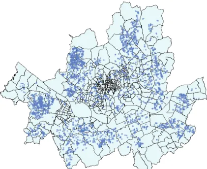
station is about 649 meters, and the typical property age of MHH is about 15 years. The average unit price of sold MHHs is 6.4 million KRW per room area (m2), and thus, the total price sold is roughly 345.6 million KRW (6.4 million KRW multiplied by 54 m2). As indicated in Figure 1, the floor level of MHH goes from the basement to the fifth floor, and units on the second floor are the most common in the MHH sales market. As for the pres- ence of elevators, 12% of the samples (377 out of 3,254 houses) are elevator-equipped MHHs. Finally, Figure 2 shows the administrative map of Seoul with sample loca- tions. The spaces where samples are not distributed are business districts or mountainous areas.
Table 1. Descriptive statistics1) (n=3,254)
Variables Min. Mean Median Max.
Room area (m2) Allocated site area (m2) Distance to subway station (m)
Age (year)
Unit price sold (million KRW per room area)
12 4 50 0 1.0
54 33 649 15 6.4
51 29 559 13 6.0
238 268 3,493 47 12.0
Figure 1. Bar chart for floors and elevators
Figure 2. Multi-household house locations (samples)
2) Explanatory variables
Variables affecting the house price could be enumer- ated endlessly. From the perspective of housing demand, some important variables could include purchaser’s in- come, mortgage interest rate, and credit regulations. For housing supply, land zoning and construction costs could have a strong influence. Therefore, selecting explanatory variables must be a compromise between theory and data availability.
We employ the area of each unit which is referred to as room area (barea), the area of the site allocated to the unit (larea), the floor on which the unit is located, age of the house, the month on which the unit is sold, a dummy variable of whether an elevator is equipped in the house, and the distance to the nearest subway station as explana- tory variables (seven variables total). We believe that we include relevant variables affecting house prices in the model specification under the constraints of data collect- ability.
3) GAMLSS models
With response vector Y, and sample size n, the linear model is defined as
Y~N(μ, σ2) (1)
μ=Xβ
where X is the n×p design matrix, β is the coefficient vector, μ is the mean vector and σ2 is a vector of constant variance.
The generalized linear model (GLM) was introduced by Nelder and Wedderburn (1972), and the normal distribution for the response variable is replaced by the exponential family of distributions (denoted here as D). It includes many important distributions, such as the nor- mal, Poisson, Gamma, inverse Gaussian, etc. The GLM can be written as:
Y~D(μ, Φ) (2)
η=g(μ)=Xβ
where Φ is the dispersion parameter, η is the linear predictor and g(·) is the link function. The normal dis- tribution, used frequently to fit empirical data, might be replaced by more flexible distribution, and in our study is replaced by the exponential Gaussian distribution, which has a characteristic positive skew, and thus, is suitable for modeling the positively skewed data such as property price. The selection of optimal distribution for the re- sponse variable from different distributions is explained in section IV.
Smoothing techniques can be incorporated within the GLM framework, resulting in the term generalized addi- tive models (GAM). The GAM can be written as:
Y~D(μ, Φ) (3)
η=g(μ)=Xβ+s1(x1)+ ... +sJ(xJ)
where sj is a non-parametric smoothing function ap- plied to explanatory variable xj, for j=1,…, J. The advan- tage of the non-parametric smoothing is that the data de- termines the relationship between the predictor η=g(μ) and the explanatory variables, rather than enforcing a linear relationship. Examples of different smoothers are numerous, and we implement a P-splines smoother in GAM.
Our chosen distribution, the exponential Gaussian distribution, has three parameters: μ, the mean of the distribution; σ, a scale parameter which is related to the variance; and ν, a shape parameter which is related to the skewness of the distribution. Up til now we have modelled only μ as a function of the explanatory vari- ables, but there are occasions in which the assumption of a constant scale parameter is not appropriate; on those occasions, modelling σ as a function of the explanatory variables could be a good option. It is also true of other parameters including ν. With enough data at hand, a model with more flexibility to deal with variance and
skewness would be preferred. Thus, we can now consider a GAMLSS model and model (3) can be extended as fol- lows:
Y~D(μ, σ, ν, τ) (4)
η1=g1(μ)=X1β1+s11(x11)+ ... +s1J1(x1J1) η2=g2(σ)=X2β2+s21(x21)+ ... +s2J2(x2J2) η3=g3(ν)=X3β3+s31(x31)+ ... +s3J3(x3J3) η4=g4(τ)=X4β4+s41(x41)+ ... +s4J4(x4J4)
where D(μ, σ, ν, τ) is a four-parameter distribution and where τ is a shape parameter related to the kurtosis of a distribution. In the case of the exponential Gauss- ian distribution, there is no parameter τ, and thus it is defined as a three-parameter distribution, D(μ, σ, ν). As for parameter link functions of the exponential Gaussian distribution, the identity function for μ and the log func- tion for σ and ν are generally utilized, and thus we follow this practice in the study.
Spatial phenomena, such as house price, cannot be analyzed accurately without due attention to property location. Identical houses can be sold for different prices depending on their specific locations. Location is the first element that comes into appraiser’s mind when valuing properties, though it is frequently ignored or underesti- mated when modeling the house price. In order to incor- porate locational elements into the model specification, we use the strategy employed by De Bastiani et al. (2016) in which relevant models for μ and other parameters are selected first without taking into account the spatial structure of the data, and then we fit the intrinsic autore- gressive model (IAR) for μ. The IAR model is suitable for explaining house prices observed in geographical areas.
When we model a house price, we expect that neighbor- ing areas are priced at more similar price levels than areas further away. The IAR model captures this expectation by bringing the fitted prices of neighboring areas closer to each other.
A pure IAR model with no explanatory variable can be written as:
y=Zγ+ε (5)
where Z is an incidence matrix (Zji=1 if data point i be- longs to area j and Zji=0 otherwise), γ is a vector of spatial random effects for the areas, and where γ~N(0, σb2G−1) for a precision matrix G and ε~N(0, σe2W−1) where W is a diagonal matrix of prior weights (De Bastiani et al., 2016). The precision matrix G can be made by using the geographical coordinates of the areas. The effect of the matrix G is to bring fitted values from neighboring areas closer together. Formula (5) is incorporated additionally into the GAMLSS formula (4) to estimate μ, the mean of the distribution (a linear predictor η1), more accurately.
The spatial random effects γˆ can be calculated by using the weighted penalized least square solution
γˆ=(ZWZʹ+λG)−1ZʹWy, where λ=σe2/σb2 (6) For further details, see De Bastiani et al. (2016).
4) Fitting algorithms
Rigby and Stasinopoulos (2005) suggested two basic algorithms for fitting GAMLSS. The first, the CG algo- rithm, is a generalization of the Cole and Green (1992) algorithm, and the other is the RS algorithm, which is a generalization of the algorithm used by Rigby and Sta- sinopoulos (1996). The RS algorithm is generally faster and far more stable, so it is used in this study to find rel- evant parameters in the model.
4. Model calibration and the results
1) Model Selection
We start from a simple model; that is, a Gaussian linear model with the seven explanatory variables men- tioned above (M1 in Table 2). Then we specify a non-
Gaussian distribution for the response variable. We com- pare the fitted models with no explanatory variable from different distributions, and the distribution with the lowest Akaike information criterion (AIC) score, in this case the exponential Gaussian distribution, is chosen. We specify the exponential Gaussian distribution with the same seven explanatory variables and the fitted model is notated as M2 in Table 2. We refine M2 by introducing a non-parametric smoothing function applied to explana- tory variables (M3). Up til M3, we have modelled only μ as a function of explanatory variables, but other distribu- tion parameters such as a scale σ and a shape ν can also be modelled efficiently under the framework of GAMLSS.
Thus, we can now consider a full GAMLSS model, M4.
And finally, we arrive at M5 in which the spatial autocor- relation is taken into account additionally. The response variable is the unit price (million KRW per room area), and all the candidate models are defined by the same seven explanatory variables.
The models are fitted by the RS algorithm, and we choose the generalized R2 and the AIC as model selection measures. The generalized R2 is defined as:
R2=1- L(0) L(fitted)
⎛⎝ ⎞
⎠
2n
(7)
where L(0) is the null model (only an intercept is in- cluded in the model) and L(fitted) is the current model.
A model with the highest R2 is usually chosen as a better model. Models can also be compared by selecting the
model with the lowest generalized Akaike information criterion: GAIC=-2lˆ+k·df, where lˆ is the fitted log- likelihood function, df is the effective degrees of freedom used in the fitted model, and k is a required penalty, e.g.
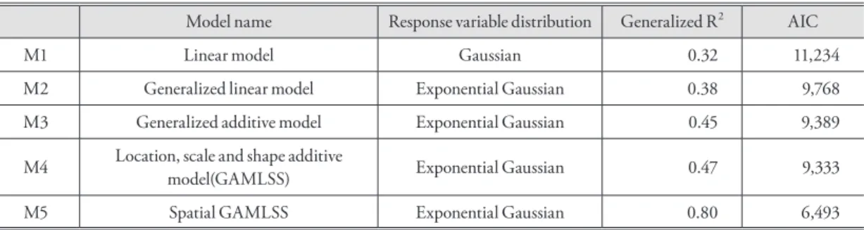
k=2 for the AIC. Table 2 shows the values of the general- ized R2 and AIC for each model.
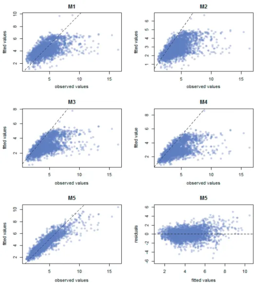
As we go from the simple model to the spatial GAMLSS model, the generalized R2 goes up, and AIC values continue to drop. This is demonstrated visually in Figure 3 where the goodness of the fit improves as it goes from M1 to M5. Therefore, we choose M5 as our final model, the specifications of which are provided in for- mula (4) to (6) of the section III.
As indicated in the two bottom panels of Figure 3, fitted values in M5 do not show a noticeable divergence from observed values, and the residuals of M5 appear to have no striking pattern. Therefore, we believe that we have no serious problem in leading a discussion based on the results of our final model.
2) Model results
We present in Table 3 the parameter estimates result- ing from the final model, jointly modeling the location (μ), variance (σ) and skewness (ν), as well as the spatial structure of the data.
The response variable (the unit price of MHH) follows the exponential Gaussian distribution with parameters μ, σ and ν. Parameter link functions for μ, σ, and ν are iden-
Table 2. Model selection and criteria
Model name Response variable distribution Generalized R2 AIC
M1 Linear model Gaussian 0.32 11,234
M2 Generalized linear model Exponential Gaussian 0.38 9,768
M3 Generalized additive model Exponential Gaussian 0.45 9,389
M4 Location, scale and shape additive
model(GAMLSS) Exponential Gaussian 0.47 9,333
M5 Spatial GAMLSS Exponential Gaussian 0.80 6,493
tity, log, and log, respectively, and hence the final model can be represented as
μ= β0+pb(barea)+β1larea+pb(floor)+pb(age) +β2month+β3elevator+β4dist_to_subway log (σ)= γ0+ γ1barea+γ2dist_to_subway log (ν)= δ0+ δ1age+δ2dist_to_subway
The μ coefficients depend on seven explanatory vari- ables ranging from room area (barea) to distance to the nearest subway station, and the pb in front of barea, floor and age represents a P-splines smoother. These smoothing
terms were employed to capture a nonlinear relationship between the response variable and the explanatory vari- ables, and their validity and meaning will be discussed in the next section. Contrary to the μ coefficients, the σ co- efficients are explained by only two explanatory variables – the room area (barea) and the distance to the nearest subway station – to relax the assumption of constant scale (variance). The ν coefficients are modelled with the help of the age of the house and the distance to the nearest subway station to describe the skewness of the distribu- tion.
Figure 3. The goodness of the fit from M1 to M5
5. Discussion and conclusion
1) Linear effect
As shown in Table 3, the intercept for μ is 5.0585, which can be roughly interpreted as the average unit price sold of MHH in Seoul being about 5 million KRW. The coefficient for the allocated site area (larea) is estimated at 0.0214, which means that as the site area increases by one square meter, the unit price increases by about 0.02 million KRW. The coefficient for the month is estimated at 0.0126, indicating that there existed an upward trend in the sales price of MHH in 2015. The co- efficient for the presence of an elevator is 0.3611, denot- ing that the MHH equipped with an elevator commands 0.36 million KRW premium for the unit price. As for the distance to the nearest subway station, the coefficient is estimated at -0.0003, meaning that the unit price de-
creases by about 0.3 million KRW as the distance to the nearest subway station increases by about one kilometer (1,000 meters).
2) Nonlinear effect
We employ a P-splines smoother for some of the ex- planatory variables (the room area, the floor on which a unit is located, and the age of the house) in describing the location parameter μ. We utilize these three smoothing terms to capture a nonlinear relationship between the unit price and the given explanatory variables. Degrees of freedom for a smoothing term represent a level of non- linearity in relationship, and those degrees of freedom for pb(barea), pb(floor) and pb(age) are 12.9, 5.4, and 9.4, respectively. When the relationship between variables is relatively linear, then degrees of freedom for a smooth- ing term are close to the value of 1.0; otherwise, degrees of freedom increase as the relationship becomes more Table 3. Results from the final model
Estimate Standard error t-value p-value
μ coefficients
Intercept 5.0585 0.0424 119.4 0.0000
pb(barea) -0.0365 0.0005 -66.4 0.0000
larea 0.0214 0.0006 36.0 0.0000
pb(floor) 0.0554 0.0071 7.8 0.0000
pb(age) -0.0656 0.0012 -53.5 0.0000
month 0.0126 0.0026 4.8 0.0000
elevator 0.3611 0.0253 14.3 0.0000
dist_to_subway -0.0003 0.0000 -16.7 0.0000
σ coefficients
Intercept -0.0477 0.0462 -1.0 0.3019
barea -0.0153 0.0005 -30.4 0.0000
dist_to_subway -0.0001 0.0000 -2.1 0.0403
ν coefficients
Intercept -0.7370 0.0392 -18.8 0.0000
age 0.0166 0.0016 10.4 0.0000
dist_to_subway -0.0003 0.0000 -6.6 0.0000
nonlinear. Thus, degrees of freedom close to 1.0 indicate that the model does not need a smoothing term to reflect a nonlinear relationship, and the linear effect is enough to model the response variable. In our study, degrees of free- dom for the three variables are high enough, and hence it is essential to employ smoothing terms for modeling the location parameter μ.
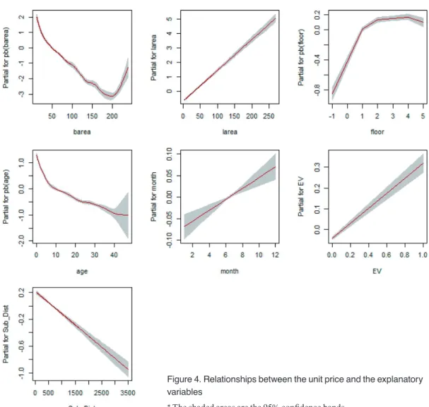
Figure 4 shows relationships between the unit price and the seven explanatory variables used for the location parameter μ, and especially, the nonlinear effects for the three smoothing terms are apparent. As shown in the first panel of Figure 4, the unit price shows a downward trend
as the room area pb(barea) goes from 0 m2 to 200 m2, but it rises abruptly after 200 m2. Diminishing unit prices for increasingly larger houses are a well-known phenomena in the property sales market, and we can see that the unit price shows a decreasing pattern until the house reaches a room area of 200 m2. When an MHH’s room area is over 200 m2 in Seoul, it is highly probable that the MHH is not an ordinary house but rather a luxurious one, and hence the unit price jumps up sharply after an MHH’s room area surpasses 200 m2.
The third panel of Figure 4 shows a nonlinear effect of the floor on the unit price. A unit located at the basement
Figure 4. Relationships between the unit price and the explanatory variables
* The shaded areas are the 95% confidence bands.
generates a considerable discount in the sales price, and a unit on the first floor shows a slight discount in sales price compared to those at the higher floors than the first floor.
There is little variation in the sales price among MHHs located between the second and fifth floor, though the units on the fifth floor show a slight downward trend. We suspect that this trend at the fifth floor might be due to 5-story MHHs that lack elevators.
The fourth panel of Figure 4 indicates a nonlinear effect of the house age on unit price. It shows an accel- erating depreciation in sales price over the first 10 years, and then a relatively gentle downward trend after that.
It denotes that MHH experiences a drastic decrease in market value over the first period since construction, and a gradual decline in value after about 10 years. In Figure 4, the rest panels not mentioned up til now show a linear effect of each explanatory variable on the unit price.
3) Spatial effect for μ
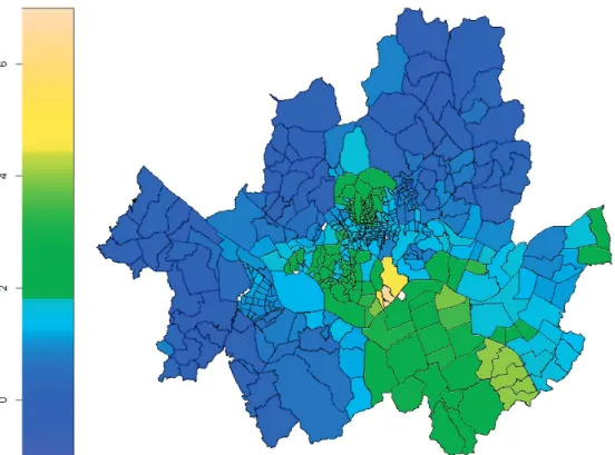
We added a spatial effect into the final model (M5) for estimating μ, the mean of the response variable dis- tribution. As indicated in formula (5) and (6), the pure error effect is notated as σe, and estimated at 32.38 in our analysis. The spatial random effect is represented as σb, and estimated at 1.07. The spatial effect might be inter- preted more intuitively by visualizing the fitted spatial effect, rather than inspecting random effect variances.
The fitted spatial effect for μ in the final model is demon- strated visually in Figure 5. The southeastern region of Seoul shows relatively high values of the fitted spatial ef- fect, which is consistent with a general expectation in the property sales market, since those areas correspond with Three Gangnam districts, an area of real estate known to be extremely expensive.
GAMLSS is well known for its capacity of not only
Figure 5. Fitted spatial effect for μ for the model M5
modeling the expected mean but also every distribution parameter (ex. scale, skewness and kurtosis) to a set of ex- planatory variables. However, Figure 5 showed that con- siderable part of property prices still remain unexplained even after modeling all the distribution parameters. The remaining component is the spatial effect, and this was efficiently captured in the spatial GAMLL model.
4) Concluding remarks
Since MHH is an emerging property type for the ap- plication of the automated valuation method in South Korea, we chose MHH as a target property for applying the hedonic price model. The hedonic price model is a common tool in estimating the property price, but it has limitations such as the lack of theoretical background for choosing a functional form, the assumption of a linear relationship between variables, and little account of spa- tial autocorrelation in model building. We suggested an alternative approach, a spatial GAMLSS model, to over- come these deficiencies in the hedonic price model fitted by regression analysis.
Our study area is Seoul and the samples obtained are 3,254 MHHs sold in 2015. We employed the room area, the allocated site area, the floor, the age of the house, the month on which the house is sold, the presence of an elevator, and the distance to the nearest subway station as the explanatory variables. We specified a GAMLSS model with the exponential Gaussian distribution for the response variable. The exponential Gaussian distribution used has three parameters μ, σ and ν, and each of them was modelled as a function of some or all the explana- tory variables given above. We also utilized a P-splines smoother for some of the explanatory variables including the room area, the floor, and the age of the house. Finally we incorporated the IAR structure into our GAMLSS model specification in order to take into account the spa- tial autocorrelation inherent in the house price. Using the generalized R2 and AIC values, we confirmed that all the
measures we took served to improve the model fit to the data. The interpretation of the effects of the explanatory variables on unit price were provided in terms of three aspects: linear, nonlinear, and spatial effect.
This study examined the prices of MHH in Seoul, and three contributions are worth noting. First, we showed that a non-normal distribution could give a better fit to the data, indicating that choosing an optimal functional form in the hedonic price model can be a quantified task free of subjective judgment. Second, we graphically illus- trated the nonlinear effects of the explanatory variables on the price of MHH, and thus suggested that capturing the nonlinear relationships in model building could give rise to a substantial benefit in the model fit results. Third, we included the IAR structure in a GAMLSS model specification, and thus proved that accounting for the spatial effect is an essential step in estimating the house price. We hope the spatial GAMLSS modeling approach provided in this study will be accepted on a wider scope, including property assessment and collateral valuation sectors, in the near future.
Note
1) The population of MHHs are 815,552 units as of 2016, and the 3,254 samples represent about 0.4% of the population. The data from the RTMS were matched with the building registry data to obtain additional information such as elevators, and illogical records (ex. an MHH unit located on the 10th floor) were removed.
References
Basu, S. and Thibodeau, T. G., 1998, Analysis of spatial auto- correlation in house prices, The Journal of Real Estate Finance and Economics, 17(1), 61-85.
Cajias, M., 2018, Is there room for another hedonic model?
The advantages of the GAMLSS approach in real estate research, Journal of European Real Estate Re- search, 11(2), 204-245.
Cole, T. J. and Green, P. J., 1992, Smoothing reference cen- tile curves: the LMS method and penalized likeli- hood, Statistics in medicine, 11(10), 1305-1319.
De Bastiani, F., Rigby, R. A., Stasinopoulous, D. M., Cysneiros, A. H. and Uribe-Opazo, M. A., 2016, Gaussian Markov random field spatial models in GAMLSS. Journal of Applied Statistics, 1-19.
De Castro, M., Cancho, V. G. and Rodrigues, J., 2010, A hands-on approach for fitting long-term survival models under the GAMLSS framework, Computer methods and programs in biomedicine, 97(2), 168- 177.
Florencio, L., Cribari-Neto, F. and Ospina, R., 2012, Real estate appraisal of land lots using GAMLSS models, Chilean Journal of Statistics, 3(1), 75-91.
Gilchrist, R., Kamara, A. and Rudge, J., 2009, An insurance type model for the health cost of cold housing: an application of GAMLSS, REVSTAT – Statistical Journal, 7(1), 55-66.
Halvorsen, R. and Pollakowski, H. O., 1981, Choice of func- tional form for hedonic price equations, Journal of urban economics, 10(1), 37-49.
Hu, W., Swanson, B. A. and Heller, G. Z., 2015, A statisti- cal method for the analysis of speech intelligibility tests, PloS one, 10(7), e0132409.
Hudson, I. L., Kim, S. W. and Keatley, M. R., 2010, Cli- matic influences on the flowering phenology of four Eucalypts: a GAMLSS approach, In Phenological Research (pp. 209-228). Springer Netherlands.
Kiffner, C., Lödige, C., Alings, M., Vor, T. and Rühe, F., 2011, Body‐mass or sex‐biased tick parasitism in roe deer (Capreolus capreolus)? A GAMLSS ap- proach, Medical and veterinary entomology, 25(1), 39 -45.
Korea, S., 2016, Korean Statistical Information Service, www.kosis.kr.
Mei, Y., Sohngen, B. and Babb, T., 2018, Valuing urban wetland quality with hedonic price model, Ecological
Indicators, 84, 535-545.
Michelson, H. and Tully, K., 2018, The Millennium Villages Project and Local Land Values: Using Hedonic Pricing Methods to Evaluate Development Projects, World Development, 101, 377-387.
Nelder, J. A. and Wedderburn, R. W. M., 1972, Generalized linear models, Journal of the Royal Statistical Society, Series A, 135: 370-384.
Rigby, R. A. and Stasinopoulos, D. M., 1996, A semi- parametric additive model for variance heterogene- ity, Statistics and Computing, 6(1), 57-65.
Rigby, R. A. and Stasinopoulos, D. M., 2005, Generalized additive models for location, scale and shape, Jour- nal of the Royal Statistical Society: Series C (Applied Statistics), 54(3), 507-554.
Rigby, R. A. and Stasinopoulos, D. M., 2006, Using the Box- Cox t distribution in GAMLSS to model skewness and kurtosis, Statistical Modelling, 6(3), 209-229.
Rosen, S., 1974, Hedonic prices and implicit markets: prod- uct differentiation in pure competition, Journal of political economy, 82(1), 34-55.
Tu, Y., Sun, H. and Yu, S. M., 2007, Spatial autocorrelations and urban housing market segmentation, The Jour- nal of Real Estate Finance and Economics, 34(3), 385- 406.
Zhang, D. D., Yan, D. H., Wang, Y. C., Lu, F. and Liu, S. H., 2015, GAMLSS-based nonstationary modeling of extreme precipitation in Beijing–Tianjin–Hebei re- gion of China, Natural Hazards, 77(2), 1037-1053.
Correspondence: Key-Ho Park, Department of Geography, Seoul National University, 1 Gwanak-ro, Gwanak-gu, Seoul, 08826, Korea (e-mail: [email protected], phone: +82-2-880- 6453)
교신: 박기호, 08826, 서울특별시 관악구 관악로 1, 서울 대학교 지리학과 (이메일: [email protected], 전화: 02- 880-6453)
Received February 15, 2019 Revised April 9, 2019 Accepted April 15, 2019