Analysis of Factors that Affect Beef Consumption in the U.S. using VAR

www.earticle.net

Analysis of Factors that Affect Beef Consumption in the U.S. using VAR

Jong-In Lee* , Jong-Tae Goh** and Hae-ShikShin***

Department of Agricultural & Resource Economics , Kangwon National University

ABSTRACT

This study focused on the factors tha t affect beef consumption in the U .8. Quarterly da ta of beef consumption , beef price , pork price , chicken price , and income from first quarter in 1970 to the third quarter in 1996 are used for the study. V AR model was used for the study using RA T8 program. Result of impulse responses , shared beef consumption responses sensitively to the shock in beef price and pork price. Whereas , a unit shock in beef consumption affects beef price. pork price , and chicken price , too. The response of chicken price was most sensitive to the shock in beef consumption.

1. Introduction

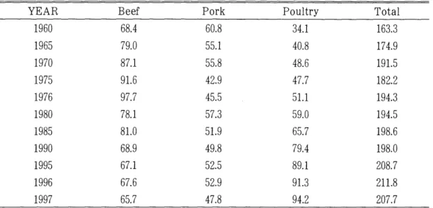
Meat consumption has changed drastically since 1960. Beef consumption increased from 68 .4 lbs/capita in 1960 to 97.71bs/capita in 1976. From the peak , beef consumption has decreased to 65.7 lbs/capita in 1997. Pork consumption has decreased since 1960 , also ,

from 60.8 lbs/capita in 1960 to 47.8 lbs/capita in 1997. However , poultry consumption has increased gradually from 34 .1 lbs/ capita in 1960 to 94.2 lbs/capita in 1997. Table 1 shows the changes of meats consumption.

These changes in meat consumption patterns are explained by relative prices for meats (Wu) , changes in relative prices (Dahlgran) and habi ts (Lambert: Chen and Veeman).

Purcell argues that price , quality , fatlcholestero l.

convenience , and time in preparation are the reasons for the change. However , Larkin argues that health information , opportunity cost of time , and the desire for convenience have influenced the change , not income or prices. Figure 1 shows retail prices for beef , por k. chicken , and turkey during 197 0- 1994.

As meat consumption patterns have changing , many researchers have tried to identify and measure structural changes in meat consumption. 80me researches show that there are structural changes in meat demand (Choi and Kim: lkerd: Braschler;

Chavas: Thurman).

As it turned out there have been structural changes in meat demand , it will be studied how each factor affects beef consumption in this study.

[Provider:earticle] Download by IP 118.70.52.165 at Monday, December 20, 2021 8:27 PM

www.earticle.net

Table 1. Per capita rneat consumption for selected years between 1960-1997 (Ibs)

Total Poultry

Pork Beef

YEAR

163 .3 34 .1

60.8 68 .4

1960

174.9 40.8

55 .1 79.0

1965

19 1. 5 48.6

55.8 87 .1

1970

182.2 47.7

42.9 9 1. 6

1975

194 .3 5 1. 1

45.5 97.7

1976

194.5 59.0

57 .3 78 .1

1980

198.6 65.7

5 1. 9 8 1. 0

1985

198.0 79 .4

49.8 68.9

1990

208.7 89 .1

52.5 67 .1

1995

21 1. 8 9 1. 3

52.9 67.6

1996

207.7 94.2

47.8 65 .7

1997

USD A ^, ERS ^, Livestock ^, D airy ^, and Poultry Situation and Outlook ^, various issues.

demand for poultry meat and the normalization and estimation of poultry meat demand equations. He established a hypothesis of stable preferences. His study showed that there was shift of demand for poultry meat in the early 1970s.

n. Review of Literature

There are many research studies about demand changes in meats. One of the approaches is the stability of meat demand.

Thurman focused on the stability of the Source

230.00 130.00 a -~m#

= _@

Q

30.00

1990 1985

1980 1975

1970

Year

-BEEF PRICE

-• -CHICKEN PRICE

- • PORK PRICE

- • TURKEY PRICE Fig. 1. Average Retail Prices for Beef , Pork , Chicken , and Turkey between 1970-1994

[Provider:earticle] Download by IP 118.70.52.165 at Monday, December 20, 2021 8:27 PM

www.earticle.net

Wohlgenant found that the mid-1970s change in beef demand was from relative prices of beef and poultry rather than preference changes. Beef demand was also more sensitive to poultry prices.

Chavas study to develop a method for investigating structural change identified structural change in beef and poultry , but not pork in the 1970s. His results explained that the price and income elasticities of beef have been decreasing , while the income elasticity of poultry has been increasing. He identified a growing influence of pork prices on beef consumption.

The study by Moschini et al. questioned whether there has been a change in structure of consumer preferences affecting U .8. beef consumption. They argued tha t the evidence of structural change is weak ,

and the decline of beef consumption may be from the change in market conditions.

For the analysis of demand changes in meats , several approaches have been taken , a linear model based on the Kalman filter ( Chavas) , a general form of the Box-Cox transforma tion (Moschini and Meilke) , a linear-in-log functional form (Thurman) , an AID8 model (Wu: Larkin) , a translog function( Choi and Kim) , and switching regressing model (Brascher). Data have also varied , quarterly data (Wu) and annual data ( Chavas: Thurman: Choi and Kim).

However , there is no study using a Vector Autoregressive (VAR) model.

ill. 않ta Consi deration and Anal ysis ^T，∞Is

1. Data and Ana/ysis Too/s

W ohlgenant emphasized the importance of relative prices ofmeats for the shift of meats demand. He also suggested the importance of other variables , for example ,

preference change , health concerns , and convenience to cook , etc. , that are assumed to affect the change of meat demand but have the problem of not being easily measured. Thus. the variables of beef consumption , beef price , pork price , chicken price , per capita income are chosen for the analysis to see how these variables affect beef consumption.

Quarterly data are used for the study ,

because quarterly data have enough information about the reactions between prices and quantities and have enough observations for the V AR model. The yearly per capita income data are divided by 4 for quarterly data. The data used are from first quarter in 1970 to the third quarter in 1996 of U.8.D .A. D ata for beef consumption , beef price , pork price , and chicken price are seasonally adjusted using PROC Xll in the 8A8 program. D ata for prices and income are deflated using CPlall urban consumer for all item. The RA T8 program was used for the main analysis.

2. VAR Mode/

An unrestricted VAR mode l, treating all variables as endogeneous (8ims) , was suggested

[Provider:earticle] Download by IP 118.70.52.165 at Monday, December 20, 2021 8:27 PM

www.earticle.net

by 8ims for short-term forecasting (Lee). but Litterman developed a Bayesian D eBenedictis explained this V AR model as an

example of a dynamic seemingly unrelated regression equations (8UR) model. The model is characterized by lagged endogeneous variables and disturbances which may be contemporaneously correlated across the equations .

8ims thought some exogeneous variables , that are categorized as exogeneous variables by previous studies , as if the list of exogeneous variables were carefully reconsidered and tested in cases where exogeneity is doubtfu l, the identification of these models might well , by Hatanakas criterion. fail. and would at best be weak.

It used to be that when expected future values of a variable were thought to be important in a behavioral equation , they were replaced by a distributed lag on that same variable (8ims). He explained that this practice had the advantage of producing uncomplicted effects on identification .

Thus , the VAR model is an alternative to large simultaneous equations models for studying the relationship among the important

procedure for estimating the V AR which grea tly improved forecasting performance (Doan). Namely , the VAR can be estimated easily with OL8 , and it is an excellent model for forecasting. Forecasting is done using the estimator after the estimation , and its a kind of chain rule of forecasting (Lee).

N. Estimation and empirical results

The price of beef , pork , chicken and income will influence each other and beef consumption. In order to estimate the influence , the Vector Autoregressive model that includes beef consumption , beef price , pork price , chicken price and income is used. We know that beef and pork are substitutes. N amely , increasing the beef price increases the consumption of pork , and increasing the pork price increases the consumption of beef. In order to examine these cases , two cases are considered. Let Xt = (dlogBC , dlogBP , dlogPP , dlogCP ,

aggregates . When 8ims developed the model dlogINCOMEJ be the vector of four it was not wellsuited for use in forecasting , variables that are estimated:

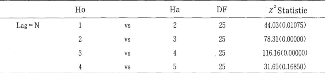
Table 2. Lag Length Tests for the VAR model

Ho Ha DF x ² Statistic

Lag=N vs 2 25 44.03 (0.01 075)

2 vs 3 25 78 .3 1 (0.00000)

3 vs 4 25 1l 6 .1 6( 0.00000)

4 vs 5 25 3 1. 65( 0 .1 6850)

[Provider:earticle] Download by IP 118.70.52.165 at Monday, December 20, 2021 8:27 PM

www.earticle.net

χ = α +β(L) I;=tχ-i + U

, Ut - N( 0 , )

where ^, BC Beef consumption BP Beef price PP Pork price CP Chicken price

INCOME Per capita income

so past prices of all four variables are permitted to predict their prices.

1. Determination of Lag Length

There are relatively few interesting hypotheses which we can test using just the estimates of a single equation from a V AR.

Most hypothesis will include more than one The VAR above is completely unrestricted , equation. The testing procedure to use is Table 3. Dependant Variable DLOGBC

Variable Coeff Std. Error T-Stat Signif.

1. D BC {1} -0.068893153 0 .1 21700070 -0.56609 0.57289786

2. D BC{2} 0 .1 12481555 0 .1 20050078 0.93696 0.35156683

3. DBC ^{3} -0.094524624 0 .1 22269719 -0.77308 0 .4 4172354

4. D BC{4} -0.042054941 0 .1 21476238 -0 .3 4620 0.73009089

5. D BP {1} -0.023156360 0.011728245 -1. 97441 0.05174314*

6. D BP{2} 0.011083923 0.012309851 0.90041 0 .3 7057092

7. DBP{3} 0.003557316 0.012436205 0.28605 0.77557384

8. D BP{4} -0.009399625 0.012624137 -0.74458 0 .4 5868307

9. DPP {1} 0ι.018019761 0.011152421 1. 61577 0 ^.1 1003239

10. DPP{2} -0.017200566 0.013550835 -1. 26934 0.20795623

1 1. D PP{3} 0.010151877 0.013874196 0.73171 0 .4 6645782

12. DPP{4} 0.001494753 0.012660888 0 .1 1806 0.90631185

13. D CP ^{1} 0.005023815 0.017764073 0.28281 0.77804578

14. D CP{2} 0.000660081 0.017978597 0.03671 0.97080274

15. D CP{3} -0.016831008 0.018115495 -0.92909 0α.35560061

16. D CP{4} 0.018381286 0.017454344 ^1. 05311 0.29542349

17. DINCOME ^{1} -0.000837842 0.001139621 -0.73519 0 .4 6434517 18. D INCOME{2} -0.001261648 0.001145936 -1. 10098 0.27416813 19. D INCOME {3} -0.000586522 0.001147392 -0.51118 0.61061692 20. D INCOME{4} -0.001591337 0.001163253 -1. 36801 0 .1 7509344 2 1. Constant 0 .1 26914309 0 .1 51760435 0.83628 0 .4 0545739

* 10% significant level

[Provider:earticle] Download by IP 118.70.52.165 at Monday, December 20, 2021 8:27 PM

www.earticle.net

the Likelihood Ratio. The test statistic is:

”

U γ

“

써 엠 ,

r

써 z

1 l I / l l

이 , ‘ ‘

」

T

l / l 、

where Lr and Lu are the restricted and unrestricted covariance matrices and T is the number of observations. This is asymptotically distributed as a %2 with degrees of freedom equal to the number of restrictions. C is a correction to improve small sample properties.

Using this likelihood ratio test , lag length Table 4. Dependant Variable DLOGBP

determined to be 4 (Table 2).

2. The corre/ation between variab/es

The estimates for coefficients are discussed in this section. Table 3 shows the coefficien않 for the dependant variable , beef consumption. Beef consumption itself affects negative effects but dlogBC(2). Beef consumption is affected positively by beef prices ^, dlogBP (l) and dlogBP( 4). However , all income variables have

Variable Coeff Std. Error T-Stat Signif.

1. D BC{ l} -1. 003865503 1. 410937460 -0.71149 0 .4 7882574

2. D BC{2} -2.904686514 1. 391808174 -2.08699 0.04003363**

3. D BC{3} 0.200475878 ^1. 417541721 0 .1 4143 0.88788533

4. D BC{4} 0.835655839 1. 408342454 0.59336 0.55459270

5. DBP ^{1} 0.263878906 0 .1 35972148 1. 94068 0.05577552 *

6. D BP{2} -0.260228313 0 ^.1 42715032 ^-1. 82341 0.07192989 * 7. D BP {3} 0.265401933 0 .1 44179932 1. 84077 0.06931716 *

8. D BP{4} 0.091903687 0.146358725 0.62793 0.53181330

9. DPP ^{1} 0ι.0애947η78226 0.129296299 0.73303 0 .4 6565552

10. DPP{2} 0.092352280 0 ^.1 57102465 -0.58785 0.55827007

1 1. D PP{3} 0 ^.1 74350142 0 ^.1 60851374 ^1. 08392 0.28161580 12. D PP{4} -0 ^.1 63542376 0 .1 46784809 -1 ^.1 1416 0.26850389 13. D CP {1} -0 .1 40769172 0.205948905 -0.68352 0.49623208

14. D CP{2} 0.055794469 0.208436000 0.26768 0.78962490

15. D CP ^{3} 0.163290468 0.210023133 0.77749 0 .4 3913583

16. D CP{4} -0.045038224 0.202358037 -0.22257 0.82443278

17. D INCOME ^{1} -0.009073807 0.013212266 -0.68677 0 .4 9418826 18. D INCOME{2} 0.007538742 0.013285484 0.56744 0.57198326 19. D INCOME{3} -0.006788856 0.013302365 -0.51035 0.61119455 20. D INCOME{4} -0.000002004 0.013486249 -1. 48582e-04 0.99988181

2 1. Constant 2.605610247 1.759444200 1. 48093 0.14250530

** 5% ^, * 10% significant level

[Provider:earticle] Download by IP 118.70.52.165 at Monday, December 20, 2021 8:27 PM

www.earticle.net

negative effects on the beef consumptio n.

DlogBP( 1) is the only variable that is significant.

5% significance level for dlogBC(Z) , and at a 10% significance level for dlogBP( 1), dlogBP(Z) , and dlogBP(3).

Table 4 shows the coefficients for the case of the dependant variable , beef price. Beef consumption has negative effects for dlogBC (1) and dlogBC(Z) , however , it has positive effects for dlogBC(3) and dlogBC( 4) on beef price. Coefficients are significant at a

In the case of pork price and beef consumption , beef consumption has positive effects for dlogBC(3) and dlogBC(4) , and negative effects for dlogBC( 1) and dlogBC(Z).

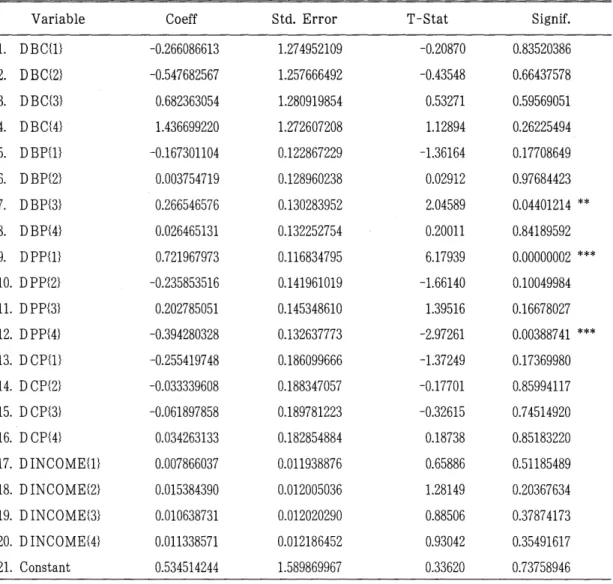
DlogBP(3) is siginficant at a 5% signifincance Table 5. Dependant Variable DLOGPP

Variable Coeff Std. Error T-Stat Signif.

1. DBC {1} -0.266086613 1. 274952109 -0.20870 0.83520386

2. DBC{2} -0.547682567 1. 257666492 -0 .4 3548 0.66437578

3. D BC{3} 0.682363054 1.28091돼9854 0.53271 0.59569051

4. D BC{4} 1. 436699220 1. 272607208 ^1. 12894 0.26225494

5. DBP {1} -0 .1 67301104 0.122867229 ^-1. 36164 0 ^.1 7708649

6. D BP{2} 0.003754719 0 .1 28960238 0.02912 0.97684423

7. D BP{3} 0.266546576 0 ^.1 30283952 2.04589 0.04401214 **

8. DBP{4} 0.026465131 0 ^.1 32252754 0.20011 0.84189592

9. DPP {1} 0.721967973 0.116834795 6 .1 7939 0.00000002 ***

10. DPP{2} -0.235853516 0ι.1 41961019 -1. 66140 0 .1 0049984 1 1. DPP{3} 0.202785051 0 .1 45348610 1. 39516 0 ^.1 6678027 12. D PP{4} -0 .3 94280328 0 .1 32637773 -2.97261 0.00388741 ***

13. D CP ^{1} -0.255419748 0.186099666 -1. 37249 0 .1 7369980 14. D CP{2} -0.033339608 0 .1 88347057 -0 .1 7701 0.85994117 15. D CP{3} -0.061897858 0 .1 89781223 -0.32615 0.74514920 16. D CP{4} 0.034263133 0 .1 82854884 0 .1 8738 0.85183220 17. DINCOME {1} 0.007866037 0.011938876 0.65886 0.51185489 18. D INCOME{2} 0.015384390 0.012005036 1. 28149 0.20367634 19. D INCOME{3} 0.010638731 0.012020290 0.88506 0 .3 7874173 20. D INCOME{4} 0.011338571 0.012186452 0.93042 0.35491617

2 1. Constant 0.534514244 1. 589869967 0.33620 0.73758946

*** 1 %, ** 5 % , * 10 % significant level

[Provider:earticle] Download by IP 118.70.52.165 at Monday, December 20, 2021 8:27 PM

www.earticle.net

leve l. and dlogPP (1) and dlogPP( 4) are dlogBC (1) on income. Where as income negatively affects to beef consumption in Table (3) , dlogBC(2) , dlogBC(3) , and dlogBC(4) affects positively to income. DlogBC( 1), dloglNCOME

(1), dlogINCOME(2) , dlogINCOME(3) , and

constant are signjficant at a 5% leve l. and dlogCP(2) and dlogINCOME(4) has signjficant at 10% the leveUTable 7).

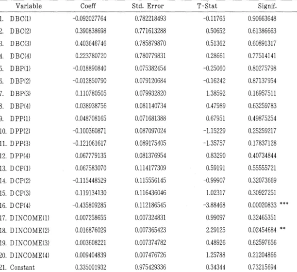
sign표Ïcant at a 10% sign표'icant leve l. (Table5) Table 6 shows the case when chicken price is the dependant variable. In this case beef consumption has positive effects for dlogBC( l).

In the case of income and beef consumption ,

beef consumption has positive effects for

Table 6. Dependant Variable DLOGCP

Variable Coeff Std. Error

1. D BC{ l} -0.092027764 0.782218493 2. D BC{2} 0 .3 90838698 0.771613288 3. D BC{3} 0 .4 03646746 0 .7 85879870

4. D BC{4} 0.223780720 0.780779831

5. D BP {1} -0.018890840 0.075382454 6. D BP{2} -0.012850790 0.079120684 7. DBP ^{3} 0 .1 10780505 0.079932820

8. D BP{4} 0.038938756 0.081140734

9. DPP ^{1} 0ι.0487깨08165 0.071681388 10. D PP{2} -0.100360871 0.087097024 1 1. D PP ^{3} -0 .1 21061617 0.089175405 12. D PP{4} 0.067779135 0.081376954 13. D CP {1} 0.067583070 0 .1 14177309 14. D CP{2} -0 ^.1 15448529 0 ^.1 15556145 15. D CP{3} 0 .1 19134130 0 .1 16436046 16. D CP{4} -0 ^.4 35809285 0 ^.1 12186545 17. D INCOME {1} 0.007258655 0.007324831 18. D INCOME{2} 0.016876029 0.007365423 19. D INCOME{3} 0.003608221 0.007374782 20. D INCOME{4} 0.009404839 0.007476726 2 1. Constant 0.335001932 0.975429336

*** 1 %, ** 5% ’ * 10% significant level

T-Stat Signif.

-0 .1 1765 0.90663648 0.50652 0.61386663 0.51362 0.60891317 0.28661 0.77514141 -0.25060 0.80275798 -0 .1 6242 0.87137954 1. 38592 0 .1 6957511 0 .4 7989 0.63259783 0.67951 0 .4 9875254 -1. 15229 0.25259217 -1. 35757 0 .1 7837128 0.83290 0 .4 0734844 0.59191 0.55555721 -0.99907 0.32073669 1. 02317 0 .3 0927251 -3.88468 0.00020833 ***

0.99097 0.32465351 2.29125 0.02454684 **

0 .4 8926 0.62597656 1. 25788 0.21204866 0.34344 0.73215694

[Provider:earticle] Download by IP 118.70.52.165 at Monday, December 20, 2021 8:27 PM

www.earticle.net

Table 7. Dependant Variable DLOGINCOME

Variable Coeff Std. Error T-Stat Signif.

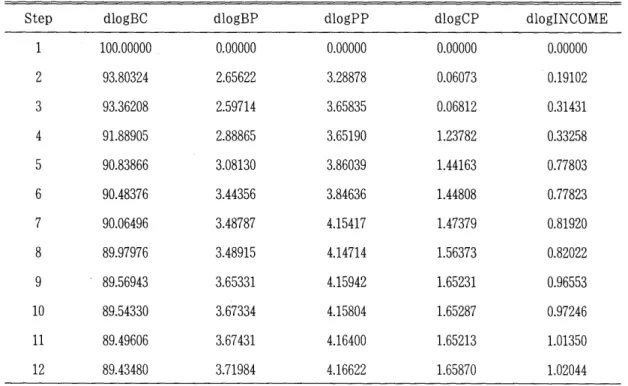
1. DBC {1} -13.57335611 6.61480516 -2.05197 0.04340327 **

2. D BC{2} 2 .4 5789456 6.52512259 0.37668 0.70739510

3. DBC {3} 1. 82858022 6.64576748 0.27515 0.78390196

4. D BC{4} 2.01153994 6.60263917 0.30466 0.76140883

5. DBP {1} -0 .1 3730795 0.63746926 -0.21540 0.83000049

6. DBP{2} -0.24422154 0.66908148 -0 .3 6501 0.71605515

7. DBP{3} 0 .4 0792089 0.67594928 0.60348 0.54787664

8. DBP{4} 0 .1 1548721 0.68616397 0 .1 6831 0.86676016

9. DPP {1} -0.29943044 0.6야061η7132 -0.49397 0.62266427

10. D PP{2} -0 .4 1691651 0.73653314 -0 .5 6605 0.57292294

1 1. D PP{3} 0.08692712 0.75410890 0 .1 1527 0.90851537

12. DPP{4} -0.54029116 0.68816155 -0.78512 0 .4 3467213

13. D CP {1} 0.85136180 0.96553669 0.88175 0.38052122

14. D CP{2} 2.92058686 0.97719677 2.98874 0.00370748 ***

15. D CP{3} -0.60160124 0.98463762 -0.61099 0.54291868

16. D CP{4} 0 .4 6215430 0.94870186 0 .4 8714 0.62747212

17. D INCOME{ l} -0 .1 4588201 0.06194220 -2 .3 5513 0.02093554 **

18. D INCOME{2} -0 .1 4728657 0.06228546 -2.36470 0.02043717 **

19. D INCOME ^{3} -0.15669859 0.06236460 -2.51262 0.01396838 **

20. D INCOME{4} 0.82520584 0.06322669 13.05154 0.00000000 ***

2 ^1. Constant 2 ^1. 51257474 8.24868636 2.60800 0.01084088 **

*** 1% , ** 5% ^’ * 10% significant level

3. 1mρulse res J) onse

According to San u tkepohl and Reimers also explain the impulse response as a common tool for investigating the interrelationships

also explained that it is used to gain a better understanding of the main channels of influence in the variables. L

1 t is assumed tha t if there is a perturbation of one standard innovation in the V AR , which influences all variables in the V AR by a chain reaction. In this section , these reactions will be considered.

among the variables in a dynamic model .tos (1 995) , An impulse response function describes the response of the system of variables to an unanticipated unit shock in any one of the variables. He

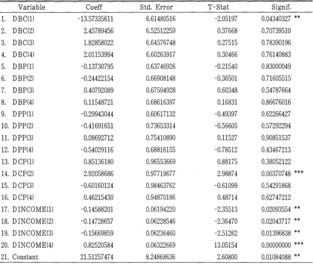
Fig. 2 Shows the responses of beef consumption to the shock in beef price ,

[Provider:earticle] Download by IP 118.70.52.165 at Monday, December 20, 2021 8:27 PM

www.earticle.net

a. Responses of beef consumption to the shock in beef price

b. Responses of beef consumption to the shock in pork price

~.: 1^ --

Ii'、'--""느~ ~----=~--~======~~~~~~~~~ ____________ ^~ __________________ ^J

-0 션 뽀삼쉰월박천컸폐옆꿇뒀갚앓앓갚찮h죠 i

c. Responses of beef consumption to the shock in chicken price

0.1 뉴ι←→ ^{• - - - - -} j

~ ~ J、~;;._^~~n. ^~~a

맏논""，，--1'\

^"τττ-::-::L

:;:; i

’

“

d. Responses of beef consumption to the shock in income

0%; 「썼

•--- 갱

Fig. 2. Responses of beef consumption to the shock in beef price. pork price. chicken prices.

and income

pork price. chicken prices. and income. Axis Y means the response and axis X means time period. namely quarter. The bold line is the response of beef consumption. and the two thin lines are estimated two standard error bounds.

When there is a unit shock in beef price.

pork price. chicken price. and income. beef

consumption respond sensitively to the shock in beef price and pork price during the 2nd term. After the second term. the responses of beef consumption decreased gradually while the responses repeat increasing and decreasing (Fig. 2. a and b).

Only Fig 2. b has a significant effect.

Fig. 3 explains the case of the responses

”

--

[Provider:earticle] Download by IP 118.70.52.165 at Monday, December 20, 2021 8:27 PM

www.earticle.net

a. Responses of beef price to the shock in beef consumption

b. Responses of beef price to the shock in pork price

c. Responses of beef price to the shock in chicken price

d. Responses of beef price to the shock in income

Fi g, 3. Responses of beef price to the shock in beef consumption , pork price , chicken price , and income

of beef price to the shock in beef consumption , pork price , chicken prices , and income. In this case , only Fig. 3. a has significant effect , but the others dont. As there is a unit shock in beef consumption ,

beef price increased during the first 5 terms ,

after that the response settled towards equilibrium (Fig. 3. a). The response of beef price increased first one term when

there is a shock in pork price. However , the responses decreased during first term when there are shocks in chicken price and income. The response of beef price responded most sensitively when there is a shock in beef consumption.

In Fig. 4 the responses of pork prices are sensitive to the shock in beef consumption ,

beef price , chicken price , and income. The

[Provider:earticle] Download by IP 118.70.52.165 at Monday, December 20, 2021 8:27 PM

www.earticle.net

a. Responses of pork price to the shock in beef consumption

b. Responses of pork price to the shock in beef price

~kJi}i(--~--- ^]

: jY얻Y41뚱캡밥깐킴릎갱룹찮꿇했텔했꿇헬꿇찮찮않꿇꿇

c. Responses of pork price to the shock in chicken price

f깐~

‘

l ~’-’’

2꽃!판륜二깐뀐합감덮화릎갚꿇찮꿇옆옆건캡6

d. Responses of pork price to the shock in income

1.5

0.5 0

-0.5 10 11 12 13 14 15 16 17 18 19 20 21 22 23 24 25 26 27 28 29 30 31 3233 34 3 -1

Fig. 4. Responses of pork price to the shock in beef consumption , beef , chicken prices ,

and income

response to the shock in beef price is sensitive during first 3 terms , and then , the

consumption , beef price , pork price , and income. It is especially sensitive to the effect is reduced gradually. This case was shock in beef price. The response of most sensitive for response of pork price ,

and it has the only significant effect.

In case of the responses of chicken price to the shock in beef consumption , beef price , pork price , and income , chicken price response sensitively to the shock in beef

chicken price to the shock in beef price ,

pork price , and income has significant effects (Fig. 5 ),

Fig. 6. explains the responses of income to the shock in beef consumption , beef price , pork price , and chicken price. In this case the

[Provider:earticle] Download by IP 118.70.52.165 at Monday, December 20, 2021 8:27 PM

www.earticle.net

3. Responses of chicken price to the shock in beef consumption

T 냐ε~====~=----률겨

-終얹펠헬펴찮옆認21같23갚25ιGε~과;고33넓

b. Response of chicken price to the shock in beef price

2

c. Responses of chicken price to the shock in pork price

0 4

깅

d. Responses of chicken price to the shock in income

0.: ~ /'\.

~ 1ι/삿슨숫~←~→~‘-→←{《-(; i

-0.5 덮찮순쉰중감r11뀔꿇피힐캡피힘갱깅핫꿇;앓꽤파윌찮짧:;37 꿇

Fig. 5. Responses of chicken price to the shock in beef consumption , beef price , pork price , and income

responses repeat same pattern unexpectedly over time.

4. Variance decomoositions (VD)

Variance decomposition is used to gain a better understanding of the main channels of influence in the variables. N amely it is explained as a k-step ahead forecast error

variance and percentages attributed to innovations in each of the variables (Santos 1996 ), Thus , the sum of the variables should be 100.

In Table 8 , the dlogBC decreased gradually , but dlogINCOME increased gradually as the time horizon increased.

However , dlogBP and dlogPP are increased suddenly from step 2. Table 8 means that - 200-

[Provider:earticle] Download by IP 118.70.52.165 at Monday, December 20, 2021 8:27 PM

www.earticle.net

a. Responses of income to the shock in beef consumption

~~ 1

_./'\.닝

1~ t: ^/.::.•(\ ~\ ..c:::::λ\/-τ‘\~~\/느(\/~V ___ -~V' ^__ I

-1u _。， §←꺼~~ν?언M낮얀M낮(νhkSM찮랬E낯잖잖후 ...

^’

^{。 、ν}

^.c.

.c.

.c.

7iJI'.c..:>.c. 약

、'v' ‘

-20 ....

b. Responses of income to the shock in beef price

c. Responses of income to the shock in pork price

1꺼? 듀二~든돈누듀논누」는~누←---든5」」펀 날 타γ장했받쓸쓸{닙끓등깜꾀치뚫깐짧품렘밥i따맺짧덮맺훌닮뭔앓잃묶옳

-2깅~L‘‘‘‘-’‘‘‘-‘‘-

d. Responses of income to the shock in chicken price

10 냥.스f슷간;파

‘~ r • ; 、=←~、음듀~‘~ξ」순~뉴~듀걷sξ도~효

:;; LL4 ^‘

Fig. 6. Responses of income to the shock in beef consumption , beef price , pork price ,

and chicken prices

although they are not large , dlogBP and dlogPP is dlogPP. DlogPP gradually decreases ,

dlogPP affect dlogBC more than dlogCP dlogBC seems to not be changed , but dlogCP

and dlogINCOME. and dlogINCOME increased as the horizon is

For dlogBP , dlogBP VD reduced increased.

gradually as step increased , while dlogBC changed little. However , dlogPP , dlogCP ,

and dlogINCOME gradually increased.

DlogBC affects dlogBP very much , but dlogINCOME has little effect (Table 9).

In Table 10 , the largest factor to affect

Table 11 shows the VD in dlogCP. D logCP is affected more by dlogBP and dlogPP than for previous cases. DlogCP decreases gradually ,

while dlogPP and dloglNCOME increased.

DlogBC and dlogBP changed little.

In Table 12 , dlogINCOME decreasd gradually ,

[Provider:earticle] Download by IP 118.70.52.165 at Monday, December 20, 2021 8:27 PM

www.earticle.net

Table 8. Decomposition of Variance of forecast errors in DLOGBC

Step dlogBC dlogBP dlogPP dlogCP dlogINCOME

100.00000 0.00000 0.00000 0.00000 0.00000

2 93.80324 2.65622 3.28878 0.06073 0 .1 9102

93 ^.3 6208 2.59714 3.65835 0.06812 0.31431

9 ^1. 88905 2.88865 3.65190 1. 23782 0 .3 3258

5 90.83866 3.08130 3.86039 ^1. 44163 0.77803

6 90 .4 8376 3 .4 4356 3. 84636 1. 44808 0.77823

7 90.06496 3 .4 8787 4 .1 5417 1. 47379 0.81920

8 89.97976 3 .4 8915 4 .1 4714 1. 56373 0.82022

9 89 .5 6943 3.65331 4 ^.1 5942 ^1. 65231 0.96553

10 89.54330 3.67334 4 ^.1 5804 1. 65287 0.97246

11 89 ^.4 9606 ^3. 67431 4 .1 6400 1. 65213 1. 01350

12 89 .4 3480 3.71984 4 .1 6622 1. 65870 1. 02044

Table 9. Decomposition of Variance of forecast errors in DLOGBP

Step dlogBC dlogBP dlogPP dlogCP dlogINCOME

18 .4 1092 8 1. 58908 0.00000 0.00000 0.00000

2 20.28687 78.81974 0.29458 0 ^.4 3833 0 ^.1 6047

3 2 ^1. 76454 77.23514 0.32994 0 ^.4 2691 0.24347

4 22.08736 75.71100 0.98287 0.99559 0.22318

5 2 ^1. 27872 76 ^.4 6735 1. 06244 0.97178 0.21971

6 20.96087 76.05717 1. 80545 0.95863 0.21788

7 20.89822 75 .4 7368 2 .1 2775 1. 09005 0 .4 1030

8 20.68032 75.64619 2 ^.1 2487 1 ^.1 3110 0 .4 1753

9 20.59441 75 .4 5425 2 ^.3 8331 1. 13982 0 .4 2822

10 20.64307 75.32604 2 ^.4 0049 1. 17850 0 .4 5190

11 20.53513 75.23283 2 .4 7212 1. 18125 0.57868

12 20.52928 75.21042 2 .4 7474 1. 18126 0.60431

[Provider:earticle] Download by IP 118.70.52.165 at Monday, December 20, 2021 8:27 PM

www.earticle.net

Table 10. Decomposition of Variance of forecast errors in DLOGPP

Step dlogBC dlogBP dlogPP dlogCP dlogINCOME

2.24777 12.21961 85.53262 0.00000 0.00000

2 1. 63407 8.80495 88 .1 7872 1. 26549 0 .1 1676

3 1. 56420 9 .1 0320 86.57251 1. 94176 0.81833

4 1. 82491 14 .1 7239 8 1. 01292 1. 87993 1. 10984

5 2 .1 5307 15 .1 4891 79 .4 7569 1. 93131 1. 29101

6 2.08106 14.89970 79.55014 2 .1 6607 1. 30304

7 2 .1 1312 14.82375 78.50665 3 .1 9873 1. 35775

8 2.07347 14.89218 78.27952 3 .4 2073 1. 33411

9 2.03174 15 .1 5199 77.84648 3.66218 1. 30762

10 2 .1 0593 15 .1 3865 77.74821 3.70233 1. 30489

11 2.10297 15 .1 9205 77.58907 3.79498 1. 32093

12 2.09800 15.26601 77 .4 6164 3.85306 1. 32130

Table 11. Decomposition of Variance of forecast errors in DLOGCP

Step dlogBC dlogBP dlogPP dlogCP dlogINCOME

3.73147 1 1. 86972 9.82532 74.57350 0.00000

2 3.70610 1 1. 73143 10 .4 8105 73.71752 0.36390

3 4.72478 12.05144 1 1. 69550 69 .3 4610 2 .1 8218

4 4 .4 0214 12.34700 15.82815 65 .4 1256 2.01015

5 4 .1 3781 1 1. 58383 16 .3 7244 66.05124 1. 85468

6 4.09022 1 1. 88613 16 .4 8700 65 .7 0149 1. 83516

7 4 .5 1434 11.65680 16 .1 6513 65.81716 1. 84657

8 4.73582 1 1. 51778 17.64036 64.23794 1. 86810

9 4.69348 1 1. 37979 18.24570 63.83445 1. 84659

10 4.68436 1 1. 41620 18.21360 63.82158 1. 86427

11 4.66879 1 1. 49158 18.05556 63.58458 2.19949

12 4.66516 1 1. 49002 18 .1 7064 63 .4 4377 2.23042

[Provider:earticle] Download by IP 118.70.52.165 at Monday, December 20, 2021 8:27 PM

www.earticle.net

Table 12. Decomposition of Variance of forecast errors in DLOGINCOME Step dlogBC

1 0.79642 2 6.94133 3 6 .4 8595 4 6 .4 1845 5 5.63833 6 8.53858 7 8.36238 8 8.22880 9 7.20333 10 9.28653 11 9 .1 4428 12 9.01082

dlogBP 0 .4 0592 0 .4 1155 0.82167 0.86762 0.50459 0.52551 0.88399 0.88527 0.71213 0.68145 0.90017 0.93300

but dlogBC , dlogPP and dlogCP increased suddenly from step 2 , step5 and step 3 each.

돼e effects of other variables to dlogINCOME are not large as previous cases.

V. Summary and Conclusions

Result of impulse responses , shared beef consumption responses sensitively to the shock in beef price and pork price.

Whereas , a unit shock in beef consumption affects beef price , pork price , and chicken price , too. The response of chicken price was most sensitive to the shock in beef consumption.

From the analysis of variance decomposition , it turned out that dlogBP and dlogPP affects dlogBC more than dlogCP and dlogINCOME ,

and dlogBC affects dlogBP more than other variables for variance decomposition in dlogBP.

However , the effects of dlogBC were not large

dlogPP dlogCP dlogINCOME

0.31084 0.28683 98 .1 9999

0 .3 0073 0.83304 9 1. 51335

0.35340 7.69906 84.63992

0.35951 8.22687 84 .1 2755

2.36839 4.88668 86.60201

3 .1 0942 4.67112 8 3. 15537 3.02675 5 .3 3482 82 .3 9206

3.03812 5.68132 82 .1 6650

2.74779 4 .4 3608 84.90067

2.62965 4.24363 83 .1 5875

2.69617 4.72242 82.53696

2 .7 4167 5.06623 82.24828

for dlogPP and dlogCP. Whereas , the effects of dlogBC , dlogBP , dlogPP , and dlogCP are not large for dlogINCOME.

Some responses show that they do not have significant effects for impulse response analysis , and only a few coefficients were statistical1y significant for correlation analysis.

These may be caused by data limitation.

More careful consideration of data and variables are needed for further study.

References

1. Braschler , Curtis. 1983. Th e Changing Demand Structure for Pork and Beef in the 197 0s:

Implications for the 198 0s. Southern Journ aJ of Agr ic uJ tural Economics , December , p105.

2. Bureau of Labor Statistics Data , 파파피L

146 .1 42 .4 .24/ cgi-bin/survevmost.

3. Chavas , Jean-Paul. 1983. Structural Change

[Provider:earticle] Download by IP 118.70.52.165 at Monday, December 20, 2021 8:27 PM

www.earticle.net

in the Demand for Mea t. American Journal of Agricultural Economics 65: 148-53.

4. Chen. P. Y. and M. M. Veeman. 199 1.

An Almost 1deal D emand Analysis for Meats with

System Habit Formation and Structural Change.

Canadian Journal of Agricultural Economics. Vol 39: pp223-35.

5. Choi. Seungmook and Sosin Kim. 1990.

Testing for Structural Change: The D emand for Meat. American Journal of Agricultural Economics. February p227.

6. D ahlgran. Roger A. 1987. Complete Flexibility System and the Stationarity of U.S. Meat D emands. Western Journal of Agricultural Economics : 152-63.

7. DeBenedictis. L.F. 1997. A Vector Autoregressive Model of the British Columbia Regional Economy. Appli

ed Economics 29: 877 -888.

8. Doan. T.A. RATS: Users Manual. Version 4. Evanston. 1L. Estima.1 992.

9. Goddard. E. W. and A.K. Amuah. 1989.

The D emand for Canadian Fats and Oils: A Case Study for Advertising Effectiveness. American Journal of Agricultural Economics 71 :741-749.

10. 1kerd. John E. March 1982. The Battle among Beef. Pork and Poultry for the Consumer ^’ s Meat D ollar. D epartment of Agricultural Economics. Oklahoma State University. Oklahoma State University Agricultural Economics Paper 8233.

1 1. Larkin. Sherry L. 1990. D omestic Meat Demand Structure Shifts due to Changing Household Characteristics. The University

of Arizona. Master Thesis.

12. Lee. J-W. 1994. Econometrics , Korean.

Seoul. Korea. Bak YoungSa.

13. Ltkepohl. Helmut and Hans-Eggert Reimers.

1992. 1mpulse response analysis of cointegrated systems. Journal of Economic Dynamics and Control. Vol16:53-78.

14. Moschini. Gincaro and Karl D. Meilke.

1984. Parameter Stability and the U.S.

D emand for Beef. Western Journal of Agricultu 'ra l EconomÍcs. Vol 9(2) :271-282.

15. Purcell. Wayne D.. 1993. Price and N on -Price F actors Affecting D emand for Meats: Emphasis on Bee f.

D epartment of Agricultural and Applied Economics. Virginia Tech University ,

Research Bulletin 4-93.

16. Santos. Rolando A. 1996. D ynamics of market structure. advertising and profitability: a V AR approach. ApplÍed Economics. Vol 27: 631-634.

17. Sims. C.A. 1980. Macroeconomics and Reality. Econometrica 48: 1-48.

18. Thurman. Walter N. 1987. The Poultry Market: Demand Stability and 1ndustry Structure. American Jouranl of Agricultural EconomÍcs p30-37.

19. Wohlgenant. M K. 1985. Estimating Cross Elasticities of Substitutio n. Westem Journal of Agricultural Economics 10:322-29.

20. Wu. Weidong. 1992. A Dynamic A1DS An alysis for U. S. Meats with Habit Formation and Structural Change. U nÍ versÍty of Nevada Reno. Master thesis.

[Provider:earticle] Download by IP 118.70.52.165 at Monday, December 20, 2021 8:27 PM