A Study on Intelligent Active Roll Angle Controller Design Analysis and Modeling Algorithm
Jung-Hyen Park*
An Intelligent active roll angle controller design algorithm is discussed. The detailed mathematical formulation and analysis are discussed, and then modeling and design method for active roll angle controller are presented.
This paper proposes a design method based upon intelligent robust controller design algorithm to control actively roll angle for improving cornering performance problems. The intelligent robust controller is designed for steady speed driving vehicle system model with representation of steering angle and yaw angular velocity parameters for cornering stability. And the detailed formulation and analysis for the objective vehicle system are investigated.
Keywords : roll angle, intelligent control, robust control, yaw angular velocity, steer angle
This paper proposes analysis, modeling and design algorithm in vehicle system to control roll angle when cornering for driving stability. The equations of motion including vehicle rolling angular motion are formulated.
The objective vehicle system is analyzed and optimal design modeling is investigated and then, intelligent robust active controller is designed for cornering stability to control roll angle with yaw angular velocity and steer angle as control input.
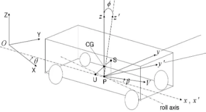
In this paper, I deal with an analysis object system based upon fixed roll axis notion theory in Fig. 1 [1-2].
In Fig. 1, X-Y plane is a driving ground surface plane and X-Y-Z are absolute coordinates. CG is the static center of gravity point of total vehicle, and P is a crossing point of roll axis and vertical line across the CG point. As point P a starting point, axis is front-to-rear axis parallel with driving ground surface plane, axis is lateral direction axis at right angles with axis, and axis is a vertical directi on axis to
axis with upper-to-lower direction; is the relative coordinates on sprung mass part. Also the point P as a standard point, it is considered as relative coordinates ′ ′ ′ on unsprung mass part.
The sprung mass is distributed symmetrically to the
*Department of Automotive & Mechanical Engineering of Silla University
접수 일자 : 2009. 2. 16 수정 완료 : 2009. 4. 25 게재확정일자 : 2009. 4. 29
plane, and S is its center of gravity point on plane. The unsprung mass is distributed on the ′ ′
plane, and its center of gravity point is U on ′ axis. In this paper, denotes the total vehicle mass; and
denote the sprung mass and the unsprung mass;
denotes length of S to axis; and denote the length of the sprung part S and unsprung part U to axis, respectively. and denote the yaw and side slip angle to the center of gravity of vehicle. and denote yaw and roll angular velocity; denote the roll angle.
And throughout in this paper, it is assumed that the vehicle was driven at the steady speed .
Fig. 1. Objective Vehicle System Coordinates The analysis model of an objective system is considered as dynamic motions of translation and rotation of its center of gravity and around that point.
In translational motion, the accelerations to the lateral directions of sprung and unsprung mass parts, the acceleration of direction and the acceleration of ′
direction can be defined as
(1)
where and denote the velocity elements of and (or ′ ) directions, respectively [3]. Assuming that side slip angle ≪ at the point P and steady speed conditions, from the relations of ≈ and ≈, follows can be obtained [4-6].
(2)
The inertia forces of sprung mass part and unsprung mass part, and is obtained as follows [2].
(3)
The inertia force of total vehicle system can be obtained as follows.
(4)
Here, , and because the CG is the center of gravity of total vehicle system, in translational motion the inertia force can be obtained as
(5) where .
In rotational motions of sprung mass part, the yawing moment around the axis to S point and rolling moment around the parallel axis to the axis can be obtained as
(6) where ⋯ are moment of inertia and product of inertia around the axis parallel to axis across the S point. And the yawing moment around the parallel axis to the ′ axis across U point on the unsprung part obtained as follow.
(7) From above, the yawing moment around (or ′) axis of total vehicle system and the rolling moment around (or ′ ) axis can be obtained as follows
(8)
because the each inertia forces of and should be adopted to U and S points. Here, under the assumption of ≪ , is the yaw moment of inertia around the vertical axis across the center of gravity point of total vehicle system, and is the rolling moment of inertia around the axis of sprung mass part, and follows are also given.
(9)
In external forces worked into the total vehicle system, its forces are considered to be lateral forces to the tires. The roll steers and of front and rear wheels can be defined as follows [2].
(10)
Because of adding steer angle of front wheel and
of rear wheel about the real steer angle , the side slip angles of front-rear-wheels are,
(11)
and cornering forces worked into front and rear wheels
and are obtained as follows
(12)
where and are tire cornering powers of each one front and rear wheel. The camber thrusts and
of front-rear-wheels can be defined as follows.
Here, and denote the camber thrust coefficients of front and rear wheels, respectively.
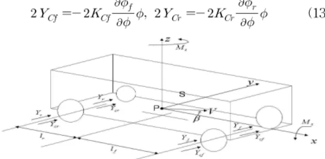
(13)
Fig. 2. External Forces into Objective System In Fig. 2, the total external forces to the lateral direction can be obtained as follows.
(14)
Also the yawing moment around axis and yawing moment around axis about to the total external forces are defined as follows.
(15)
(16) In Eq. (16), and denote the total roll stiffness of front-rear suspensions and equivalent viscous friction coefficient of rolling motion, respectively.
Based on the objective system analysis, the relations of lateral forces, yawing and rolling moments can be considered as follows.
(17)
From Eq. (5), Eq. (8) and Eqs. (14)-(16), the equations of the vehicle motion can be obtained as follows.
(18)
(19)
(20)
Those are considered that is yawing moment of inertia of total vehicle and is rolling moment of inertia around roll axis of the vehicle where axis and roll axis can be considered as same location. Finally, the following dynamic equations are derived
(21)
(22)
(23)
where
(24)
To design intelligent robust yaw angle control system, Eqs. (21)-(23) are represented by
(25)
where
(26)
Here, and are control input coefficients. The matrix representations of Eq. (24) become as follows.
(27)
That is; ⇕
(28)
In this paper, the control system is designed with the
intelligent robust ∞ control to improve the cornering stability. The state space equation form of Eq. (26) can be modeled and expressed as
(29)
where and denote roll angle and roll angular velocity as the state system variables, and yaw angular velocity and steering angle as control input; and denote measured output and controlled output of the control system. denotes external forces elements as disturbances input. System design variables and matrix parameters become as follows.
Intelligent robust ∞ control problem is to find a controller such that the closed-loop system is internally stable and the following ∞ norm condition,
∥ ∥∞ is satisfied. is the transfer function from the disturbance input to the controlled output in the closed-loop system, is a prescribed positive number [7-8]. In order to design robust ∞ controller for controlled objective system, it is assumed that the following two Riccati equations about to and positive-definite matrices
(30)
(31)
have two solutions of positive and
. Then there exists controller such that the closed-loop system of objective system is internally stable and the above ∞ norm condition is satisfied [9-10]. In this paper, one of the intelligent robust controllers can be defined as follows
(32)
where
Fig. 3. Bode Frequency Response of Roll Angle
Fig. 4. Bode Response of Controlled plant
The bode frequency responses of design objective plant yaw angle and ∞controller are shown in Fig. 3-4. In detail numerical simulation specifications, those were set that the vehicle mass =100 slugs, =90 slugs, =10 slugs, =2500 slug·ft2, =10 ft, =5.5 ft, , =9000, 8900 lb/rad, =520 slug·ft2, =1.2 ft, =100 ft/s, and
= 8100 lb·ft/rad. Also it is considered that
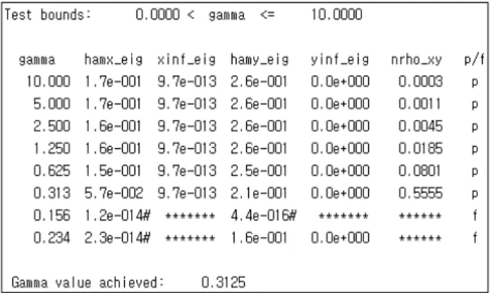
. The result of -iteration [11] calculation to solve the robust ∞ control problem in this paper is shown as Table 1.
Table 1. Result of -iteration
In this paper, I dealt with a design method based upon intelligent robust ∞ control system design algorithm to control actively roll angle for improving cornering performance problems. The intelligent robust controller was designed for steady speed driving vehicle system model with representation of steering angle and yaw angular velocity parameters for cornering stability.
The detail formulation and analysis for the objective vehicle system were investigated and expected small value was achieved.
[1] L.Segal Theoretical prediction and experimental substantiation of the response of the automobile to steering control, Proc. of I. Mech. E. (A.D.), 1957.
[2] M.Abe, Automotive dynamics and control, TDU-Press, 2008
[3] G. W. Housner and D. Hudson, Applied mechanics dynamics, D. Van Nostrand Company, 1959.
[4] E. I. Ono, "A Study on the Integrated Control of Automotive Dynamics", Journal of Systems, Control and Information, Vol. 49, No. 6, pp. 205-210, 2005.
[5] The Vehicle System Dynamics and Control. JSME, Yokendo, 1999.
[6] A. V. Zanten and R. Erhart, “The Vehicle Dynamics Control System of Bosch”, SAE PT, vol.
57, pp.497~514, 1996.
[7] J. H. Park, “A study on adopting intelligent control system in active suspension equipment,” Journal of The Korea Society of Computer and Information, vol. 12, No. 3, pp. 287–293, 2007.
[8] J. H. Park and W. S. Ahn, “∞ Yaw‐Moment Control with Blake for Improving Driving Performance and Stability” Proc. of IEEE/ASME Conference on Advanced Intelligent Mechatronics September 19‐23, Atlanta, USA, 1999.
[9] J. H. Park, “A study on active suspension control system in vehicle bouncing and pitching vibration for improving ride comfort,” Journal of The Korea Society of Computer and Information, vol. 12, No.
2, pp. 325–331, 2007.
[10] J. H. Park, “Combined Optimal Design with Minimum Phase System”, Journal of Control, Automation, and Systems Engineering, Vol. 10, No 2, pp. 192-196, 2004.
[11] J. Mita, ∞ Control, Shokodo Press, 1994.
Jung Hyen Park received the B.S.
degree in mechanical engineering from Pusan National University in 1992 and M.S. and Ph.D degrees in systems engineering from Kobe University in 1995 and 2000, respectively.
Joined the department of Automotive & Mechanical Engineering of Silla University in 2001. Present an associate professor. His research interests include the areas of vehicle system analysis, system modeling, system design, intelligent control system design.